DWDM Practical
guide for cracking optical interviews
![]()
DWDM Practical
guide for cracking optical interviews
![]()
INTRODUCTION
MapYourTech's Interview
Buddy Series is an initiative to help Optical Fiber Communication
Professionals increase their technical and behavioral interview skill sets
which will help them excel in their professional career.
In
this series, utmost care has been taken to include practical DWDM based
questions that are asked in related industries during current time.
Intent
is to enable optical professionals’ interest and equipping them with right
tools to excel in their career.
DWDM
(Dense Wavelength Division Multiplexing) is an interesting branch of Optical
Fiber Communication which acts as a backbone to the telecom networks delivering
high capacity and highspeed data from one end to another.
TABLE OF CONTENT
Question 1:
What is DWDM and how it works?
Question 2: What
are the basic component of DWDM link?
Question 3: What
is a transponder?
Question 4: What
are the major types of transponder used in network?
Question 5: What are the major advantages of using
coherent transponders?
Question 6: What are performance parameters on
Transponders?
Question 7: What is a multiplexer (MUX) and a
demultiplexer(DEMUX)?
Question 8: What is an Amplifier ? What are the types
of amplifier we use in a DWDM Network ?
Question 10: What is ASE and how does it affect EDFA
performance?
Question 11: What is the maximum number of EDFA's to
cascade in a DWM link and why?
Question 12: What are main advantages and drawbacks of
EDFAs?
Question 13: What are the types of Amplifiers based on
their placement in a DWDM Link?
Question 14: What is power control mode and Gain
control mode?
Question 15: What is the effect of Amplifier gain on
OSNR while reducing or increasing flat gain?
Question 16: What is gain tilt and Gain ripple?
Question 17: What is a 30 dB gain means?
Question 18: What is Raman Amplifier and how does it
work?
Question 19: What are the advantages of using Raman
Amplifier?
Question 20: What are the Noise sources in Raman
Amplifier?
Question 22: Why generally EDFA and Raman are used in
conjunction to each other?
Question 23: What are linear effects?
Question 24: What are nonlinear effects?
Question 25:
What are the types of Nonlinear effects that happens in a DWDM link?
Question 26: What is impact of linear and nonlinear
effects in DWDM network?
Question 27: How to reduce FWM impact?
Question 29: What are different types of fibers and
what is their significance?
Question 30: What are Fiber spectrum bands?
Question 31: What is Red and Blue and Red Band is
preferred over Blue in DWDM?
Question 32: What is dark fiber, dim fiber and lit
fiber?
Question 33: What are the sources of latency in
optical fiber?
Question 34: What is micro bending and macro bending?
Question 35: What is fiber characterization?
Question 37: What is PMD coefficient and its unit?
Question 40: What is cause of CD?
Question 41: What is unit of CD and CD Coefficient?
Question 42: Which are main factors for CD?
Question 43: How to mitigate CD in a link?
Question 44: What are general performance parameters
available on an Optical Amplifiers?
Question 47: What are methods to reduce CD in link?
Question 48: What is DCM or DSCM or DCU?
Question 49: What are considerations while deploying
DCM?
Question 50: What are the types of DCM in DWDM link?
Question 53: What is Optical Return Loss (ORL) in
Optical Fiber system?
Question 54: What are the major sources of ORL?
Question 55: what are the implications of ORL?
Question 56: How does reflected power affect laser
stability?
Question 58: What are the methods to help improve
ORL?
Question 59: Why it is Good to have ORL >30dB for
general fiber links?
Question 61: What is Q-factor and what is its
importance?
Question 62: What are the advantages of Coherent
Optical Transmission System?
Question 63: Why Receiver Sensitivity is so important
for optical module?
Question 64: What is attenuation in Optical fiber?
Question 65: What are the general colors of patch
cord seen in Optical environment?
Question 66: Defining Colorless, Directionless,
Contention-less flexible grid Network?
Question 67: Why Do We Need Gridless?
Question 68: What Is Coherent Communication?
Question 70: What does Tap ration means for splitter
and Coupler?
Question 71: What an OTDR can do for you?
Question 72: What is the difference between HD-FEC & SD-FEC in coherent transponders?
Question 73: Why is it preferable to put
attenuator/pad at the Receive end of Optical Module?
Question 74: How and where do we get pre and post FEC
BER?
Question 75: what are the Optical Fiber Link Design
requirements?
Question 77: What is the relationship between BER and
Q factor?
Question 78: What are the noise sources known in
Optical fiber network?
Question 79: What is resolution bandwidth?
Question 80: What is noise equivalent bandwidth?
Question 82:
Why is the BER not easy to simulate/calculate?
Question 83: What is ROADM? What problems ROADM can
solve?
Question 84: What is TVSP, and what is its effect?
Question 85:
What are the main reasons behind the fluctuation of the Q factor?
Question 86:
What is Spectral Efficiency, and what is its role in coherent technologies?
Question 87: What is the basic behind increasing SE?
Question 88: What is the main purpose of using
Coherent Detection in a system?
Question 89: How does changing modulation improves
the reach of a system?
Question 90: What are the key characteristics of
optical amplifiers?
Question 91: What are the main issues
associated with EDFA in a DWDM link?
Question 92: What are the parameters associated with
fibers in a link?
Question 93: What are the parameters associated with
optical light sources in a link?
Question 94: What are the parameters associated with
optical light receivers in a link?
Question 95: How does temperature affects EDFA
performance?
Question 96: What are
some ways to increase the capacity of an optical system?
Question 97: What is the significance of the eye
diagram?
Question 99: Why does FEC introduce latency?
Question 101: What is dBm and what are
the major conversions used in Optical Network?
Question 102: Which components and
technology is used in ROADM?
This page is left
intentionally blank
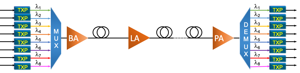
Dense Wavelength division multiplexing
(DWDM) is a technology used to combine or retrieve two or more optical signals
of different optical center wavelengths or frequencies in a fiber. This allows
fiber capacity to be expanded in the frequency domain from one channel to
greater than 100 channels. This is accomplished by first converting standard,
non-DWDM optical signals to signals with unique WDM wavelengths or frequencies
that will correspond to the available channel center wavelengths in the WDM
multiplexer and demultiplexer. Typically, this is done by replacing non-WDM
transceivers with the proper WDM channel transceivers. WDM channels are defined
and labeled by their center wavelength or frequency and channel spacing. The
WDM channel assignment process is an industry standard defined in International
Telecommunications Union (ITU-T). Then different WDM signal wavelengths are
combined over one fiber by the WDM multiplexer. In the fiber, the individual
signals propagate with minimal interaction assuming low signal power. For high
powers, multiple interactions can occur. Once the signals reach the fiber link
end, the WDM demultiplexer separates the signals by their wavelengths, back to
individual fibers that are connected to their respective equipment receivers.
Optical receivers have a broad reception spectrum, which includes all of C
band. Many receivers can also receive signals with wavelengths down to O band.
Above schematics show basic DWDM block
diagram.
DWDM components includes: -
Transponders
To convert grey or black and white signals
to colored (different frequency) signals with O-E-O mechanism.
Multiplexer
To
aggregate different channels in form of composite channel.
Amplifier
To boost signal strength so that it can
travel large distance.
Demultiplexer
To
dis-aggregate various channel coming from network to respective frequencies.
Transponder is the integrated part of WDM systems
use to transmit signal over a DWDM link. This module takes black and white or
grey signals as input on 1310nm, 1550nm or 850nm and converts those signals
into colored channels or certain frequencies in C or L band. This is achieved
by using optical-electrical-optical conversion mechanism. Transponders along
with Optical source also includes complex components that helps signal in
serialization and deserialization of frames, control and monitoring capabilities
etc.
There are two
types of transponders:
•
optical - to - electrical - to - optical (O - E -
O)
•
optical - to - optical (O - O).
The O - E - O
transponder may also act as a 3R repeater; that is, it performs signal
reshaping, retiming, and reconstitution or gain; O - E - Os are more complex
and more expensive, Because the signal is converted to electronic, an O - E - O
node allows for add - drop functionality, in addition to simple optical relay
or transponder.
The O - O
transponder, or optical relay, is technologically more attractive because it
performs direct optical - to - optical amplification using optical amplifiers
(doped fiber - based (EDFA) or semiconductor optical amplifiers (SOA)) thus
acting as an all - optical relay.
There are two
types of transponders
•
non coherent transponders
•
coherent transponders
non coherent transponders:
These
transponders involve IM/DD (Intensity Modulation/Direct Detection) technique
also known as OOK method for transmission of signal. In IM/DD the intensity, or
power, of the light beam from a laser or a light-emitting diode (LED) is
modulated by the information bits and no phase information is needed. Due to
this nature, no local oscillator is required for IM/DD communication, which
greatly eases the cost of the hardware.
coherent
transponders:
The basic idea behind
coherent detection consists of combining the optical signal coherently with a
continuous-wave (CW) optical field before it falls on the photodetector. The CW
field is generated locally at the receiver using a narrow line width laser,
called the local oscillator (LO). With the mixing of the received optical
signal with the LO output can improve the receiver performance.
The
major advantage of using the coherent detection techniques is that both the
amplitude and the phase of the received optical signal can be detected,
extracted and measured accordingly. This
method helps in sending information by
modulating either the amplitude, or the phase, or the frequency of an optical
carrier. In the case of digital communication systems, the three possibilities
give rise to three modulation formats known as amplitude-shift keying (ASK),
phase-shift keying (PSK), and frequency-shift keying (FSK)
Use of coherent detection
may allow a more efficient use of fiber bandwidth by increasing the spectral
efficiency of WDM system. Sometimes it has been seen that the receiver
sensitivity can be improved by up to 20 dB compared with that of IM/DD systems
BER, and hence the receiver sensitivity.
Usually Transponders have
following optical parameters to monitor:
|
Optical power receives. |
|
Normalized optical power receive. |
|
Optical power receive (minimum). |
|
Optical power receive (maximum). |
|
Optical power receive (average). |
|
Optical power transmit. |
|
Optical power transmit (minimum). |
|
Optical power transmit (maximum). |
|
Optical power transmit (average). |
|
Optical power receive OTS. |
|
Normalized optical power receive OTS. |
|
Optical power receive OTS (minimum). |
|
Optical power receive OTS (maximum). |
|
Optical power receive OTS (average). |
|
Differential group delay (average). |
|
Differential group delay (maximum). |
|
Code violations, OTU, near end receive. |
|
Errored seconds, OTU, near end receive. |
|
Severely errored seconds, OTU, near end receive. |
|
Severely errored frame seconds, OTU, near end receive. |
|
FEC corrections, OTU, near end receive. |
|
High correction count seconds, OTU, near end receive. |
|
Pre-FEC BER, OTU, near end receive. |
|
Pre-FEC BER (maximum), OTU, near end receive. |
|
Post-FEC BER estimates, OTU, near end receive. |
|
Q min, OTU, near end receive. This represents the Q low water mark. |
|
Q max, OTU, near end receive. This represents the Q high water mark. |
|
Q average, OTU, near end receive. This represents the average Q during the
measured interval. |
|
Q standard deviation, OTU, near end receive. This
represents the standard deviation of the Q during the measured interval. |
|
Uncorrected FEC block, OTU, near end receive. |
|
Code violations, ODU, near end receive. |
|
Errored seconds, ODU, near end receive. |
|
Severely errored seconds, ODU, near end receive. |
|
Unavailable seconds, ODU, near end receive. |
|
Failure count, ODU, near end receive. |
As
DWDM systems send signals from several sources over a single fiber, they must
be able to combine the incoming signals. This is done with a multiplexer, which
takes optical wavelengths from multiple fibers and converges them into one
beam. At the receiving end, the system must be able to separate out the
components of the light so that they can be discreetly detected. Demultiplexers
perform this function by separating the received beam into its wavelength
components and coupling them to individual fibers. Demultiplexing must be done
before the light is detected, because photo-detectors are inherently broadband
devices that cannot selectively detect a single wavelength.
Multiplexers
and demultiplexers can be either passive or active in design. Passive designs
are based on prisms, diffraction gratings or filters, while active designs
combine passive devices with tunable filters. The primary challenges in these
devices is to minimize cross-talk and maximize channel separation. Cross-talk
is a measure of how well the channels are separated, while channel separation
refers to the ability to distinguish each wavelength
Amplifiers are the modules used generally in
long haul networks to manage loss in a DWDM network. Here the signal is
directly amplified without conversion of optical signal into electrical signal
.
Optical Amplifiers amplify input light through
stimulated emission, the same mechanism that is used by lasers but only
difference is that amplifiers doesn't need feedback circuitry. It’s main
ingredient is the optical gain realized when the amplifier is pumped
(electrically or optically ) to achieve population inversion. The optical gain,
in general, depends not only on the frequency (or wavelength) of the incident
signal, but also on the local signal intensity at any point inside the
amplifier.
There are mainly two types of amplifiers used
in DWDM network and they are EDFA(Erbium doped fiber Amplifier ) and Raman
Amplifier.
EDFA:
Erbium doped fiber amplifiers makes use of
rare-earth elements (Er3+ ) as a gain medium by doping the fiber core during
the manufacturing process .Erbium-doped fiber amplifiers (EDFAs) is widely used
because they operate in the wave- length region near 1.55 μm .In EDFA,pumping
at a suitable wavelength provides gain through population inversion. The gain
spectrum depends on the pump- ing scheme as well as on the presence of other
dopants, such as germania and alumina, within the fiber core. Efficient EDFA pumping
is possible using semiconductor lasers operating near 0.98- and 1.48-μm
wavelengths. Most EDFAs use 980-nm pump lasers as such lasers are commercially
available and can provide more than 100 mW of pump power. Pumping at 1480 nm
requires longer fibers and higher powers because it uses the tail of the
absorption band ,
RAMAN:
Raman fiber uses SRS (stimulated Raman
scattering ) phenomenon which was experimentally observed by Sir Chandrasekhara
Venkata Raman in 1928.
SRS is used in silica fibers when an intense
pump beam propagates through it .With this effect the incident pump photon
gives up its energy to create another photon of reduced energy at a lower
frequency (inelastic scattering); the remaining energy is absorbed by the
medium in the form of molecular vibrations (optical phonons). Thus, Raman
amplifiers must be pumped optically to provide gain. The pump and signal beams
at different frequencies are injected into the fiber through a fiber coupler.
The energy is transferred from the pump beam to the signal beam through SRS as
the two beams co-propagate inside the fiber. Commonly counter propagation mode
is used. The gain from a Raman amplifier increases almost linearly with the
wave- length offset between signal and pump, peaking at about an 100-nm
difference, then it drops off rapidly.
The 980nm pump needs three energy level for radiation while
1480nm pumps can excite the ions directly to the metastable level .
Though pumping with 1480 nm is used and has an optical power conversion
efficiency which is higher than that for 980 nm pumping, the latter is
preferred because of the following advantages it has over 1480 nm pumping.
▪
It provides a
wider separation between the laser wavelength and pump wavelength.
▪
980 nm pumping
gives less noise than 1480nm.
▪
Unlike 1480 nm
pumping, 980 nm pumping cannot stimulate back transition to the ground state.
▪
980 nm pumping
also gives a higher signal gain, the maximum gain coefficient being 11 dB/mW
against 6.3 dB/mW for the 1.48
▪
The reason for
better performance of 980 nm pumping over the 1.48 m pumping is related to
the fact that the former has a narrower absorption spectrum.
▪
The inversion
factor almost becomes 1 in case of 980 nm pumping whereas for 1480 nm pumping
the best one gets is about 1.6.
▪
Quantum mechanics
puts a lower limit of 3 dB to the optical noise figure at high optical gain.
980 nm pimping provides a value of 3.1 dB, close to the quantum limit whereas
1.48 pumping gives a value of 4.2 dB.
▪
1480nm pump needs
more electrical power compare to 980nm.
▪
Typically, 980 nm
pumping results in a noise figure 1 dB lower than that for 1480 nm pumping.
▪
The shorter
wavelength results in less noise.
During
population inversion phenomenon and as spontaneous emission occurs in all modes
supported by the fiber (guided and unguided). Clearly, some of these photons
would appear from time to time in the same fiber mode occupied by the signal
field. Such spontaneously emitted photon perturbs both the amplitude and the
phase of the optical field in a random fashion. These random perturbations of
the signal are the source of amplifier noise in EDFAs and results in ASE.
For long haul links,
generally EDFA's are cascaded to overcome fiber losses in the link. Due to
these cascading structures, amplifier induced noise buildup and impacts the
performance of Amplifier. The ASE accumulates over many amplifiers and degrades
the optical SNR. Also, as the level of ASE grows, it begins to saturate optical
amplifiers and reduce the gain of amplifiers located further down the fiber
link. The net result is that the signal level drops further while the ASE level
increases. So, it's obvious that if the number of amplifiers is large, the SNR
will degrade so much at the receiver that the BER will become unacceptable.
Maximum number of
erbium-doped fiber amplifiers (EDFAs) in a fiber chain is
about four to six.
The rule is based on the following rationales:
1. About 80 km exists between each in-line EDFA,
because this is the approximate distance at which the signal needs to be
amplified.
2. One booster is used after the transmitter.
3. One preamplifier is used before the receiver.
4. Approximately 400 km is used before an amplified
spontaneous emission (ASE) has approached the signal (resulting in a loss
of optical signal-to-noise ratio [OSNR]) and regeneration needs to be used.
An EDFA amplifies all the wavelengths and modulated as well as
unmodulated light. Thus, every time it is used, the noise floor from
stimulated emissions rises. Since the amplification actually adds power to
each band (rather than multiplying it), the signal-to-noise ratio is
decreased at each amplification. EDFAs also work only on the C and L bands
and are typically pumped with a 980- or 1480-nm laser to excite the erbium
electrons. About 100 m of fiber is needed for a 30-dB gain, but the gain
curve doesn’t have a flat distribution, so a filter is usually included to
ensure equal gains across the C and L bands.
Advantages:
▪
Commercially
available in C band (1,530 to 1,565 nm) and L band (1,560 to 1,605) and up to
84-nm range at the laboratory stage.
▪
Excellent
coupling: The amplifier medium is an SM fiber;
▪
Insensitivity
to light polarization state;
▪
Low
sensitivity to temperature;
▪
High
gain: > 30 dB with gain flatness < ±0.8 dB and < ±0.5 dB in C and L
band, respectively, in the scientific literature and in the manufacturer
documentation
▪
Low
noise figure: 4.5 to 6 dB
▪
No
distortion at high bit rates;
▪
Simultaneous
amplification of wavelength division multiplexed signals;
▪
Immunity
to crosstalk among wavelength multiplexed channels (to a large extent)
Drawbacks:
▪
Pump
laser necessary;
▪
Difficult
to integrate with other components;
▪
Need
to use a gain equalizer for multistage amplification;
▪
Dropping
channels can give rise to errors in surviving channels: dynamic control of
amplifiers is necessary.
With the placements, there are three types of
amplifiers:
•
Booster
Amplifier
•
Pre-Amplifier
•
In-Line
Amplifier
Booster Amplifier
Main purpose of booster
amplifier is to boost the power transmitted.
A booster amplifier is
used to amplify the signal channels exiting the transmitter to the level
required for launching into the fiber link. In most applications this level is
in the range of 0-5 dBm per channel, however, it can be higher for more demanding
applications. A booster is not always required in single channel links, but is
essential in a WDM link where the multiplexer attenuates the signal channels. A
booster amplifier typically has low gain (in the range of 5-15 dB) and high
output power, typically about 20dBm for a 40 channel WDM system. The NF of a
booster amplifier is not usually a critical parameter. At the other end of a
link a pre-amplifier may be required to amplify the optical signal to the level
where it can be detected over and above the thermal noise of the
receiver.
Pre-Amplifier
These amplifiers are
commonly used to improve the receiver sensitivity. Transmission distance can
also be increased by putting an amplifier just before the receiver to boost the
received power.
A pre-amplifier should
provide high gain, often in the range of 30 dB, and have a low NF in the range
of 4-5.5 dB, in order to assure error-free detection of the signal channels.
The output power of the pre-amplifier need not be very high.
For links up to about 150
km, a booster and/or pre-amplifier are usually sufficient to ensure error-free
transmission. However, for links above 150 km the performance deteriorates to
such an extent that the signal becomes undetectable.
In-Line Amplifier
These amplifiers are used
for compensating distribution losses in local-area networks. replace electronic
regenerators. An in-line amplifier is characterized by large gain and low noise
to amplify an already attenuated signal so that it can travel an additional
length of fiber.
In-line amplifiers are
placed every 80-100 km to ensure that the optical signal level remains above
the noise floor. In-line amplifiers typically require moderate gain in the
range of 15-25 dB, and NF in the range of 5-7 dB. Output power requirements are
similar to those of booster amplifiers. While in the early days of optical
amplifiers different amplifier models had to be specifically tailored for each
of the above functions, today the technology has advanced so that a single well
designed amplifier model can perform many of the functions for typical
applications. However, there still remain challenging applications which
require specially designed amplifiers, such as very high output power boosters,
or ultra-low noise pre-amplifiers.
Power Control Mode:
When amplifier works in power control mode, it
maintains constant per channel power when desired or accidental changes to the
number of channels occur. Constant per channel power increases optical network
resilience.
Gain Control mode:
In constant gain mode, the amplifier power out
control loop performs the following input and output power calculations, where
G represents the gain and t represents time.
Pout (t) = G *
Pin (t) (mW)
Pout (t) = G +
Pin (t) (dB)
A common way
to characterize the performance of an amplifier is through its Noise figure.
The noise figure is defined as the ratio of the signal to noise ratio at
the input of
the amplifier-receiver to that at the output of the amplifier:
NF= SNR in/SNR out
The noise
figure will always be greater than one, due to the fact that the amplifier Adds
noise during the amplification process and the signal to noise ratio at the
output is always lower than that at the input. The noise figure value is
usually given in dB.
Noise output
power ASE (Amplified Spontaneous Emission) directly depends on Gain of
Amplifier. The OSNR at any point in a fiber link is equal to the signal
power divided by the noise power. If
Noise power will increase OSNR will decrease and will introduce errors in channel.
But in link
where multiple EDFA deployed, gain is set as per planning, but there is always
some margin, for gain adjustment. If you will increase Gain of first few EDFA,
as this gain will increase noise power (ASE) and this ASE will mix with Signal
power and with signal power, noise power will be amplified by downstream EDFA,
and this ASE will degrade final OSNR of channels.
The ability to control and adjust per channel
optical power equalization is a principal feature of Amplifier in network
applications. A major parameter to assure optical spectrum equalization
throughout the DWDM system is the gain flatness of erbium-doped fiber
amplifiers (EDFAs).
Effect of Gain Ripple and Gain Tilt on
Amplifier Output Power are as follows:
Gain ripple:
Gain ripple is random and it depends on the
spectral shape of the amplifier optical components.
Gain tilt:
Gain tilt is systematic and it depends on the
gain set point of the optical amplifier, which is a mathematical function that
relates to the internal design of the amplifier.
Gain tilt is the only contribution to the power
spectrum dis-equalization that can be compensated at the module level. A VOA
inside the amplifier can be used to compensate for gain tilt. An optical
spectrum analyzer (OSA) is used to acquire the output power spectrum of an
amplifier. The OSA shows the peak-to-peak difference between the maximum and
minimum power levels, and takes into account the contributions of both gain
tilt and gain ripple.
30dB gain means for every
input PHOTON there will be 1000 PHOTON's at output. That's what Gain is.
X dB is 10x/10
Raman amplifier is a
well-known amplifier configuration. This amplifier uses conventional fiber
(rather doped fibers), which may be co-or counter-pumped to provide
amplification over a wavelength range which is a function of the pump
wavelength. The Raman amplifier relies upon forward or backward stimulated
Raman scattering. Typically, the pump source is selected to have a wavelength
of around 100 nm below the wavelength over which amplification is required.
Principle of working:
As the
pump laser photons propagate in the fiber, they collide and are absorbed by
fiber molecules or atoms. This excites the molecules or atoms to higher energy
levels. The higher energy levels are not stable states so they quickly decay to
lower intermediate energy levels releasing energy as photons in any direction
at lower frequencies. This is known as spontaneous Raman scattering or Stokes
scattering and contributes to noise in the fiber.
Since
the molecules decay to an intermediate energy vibration level, the change in
energy is less than the initial received energy during molecule excitation.
This change in energy from excited level to intermediate level determines the
photon frequency since Δ f = Δ E / h. This is referred to as the Stokes
frequency shift and determines the Raman gain versus frequency curve shape and
location. The remaining energy from the intermediate level to ground level is
dissipated as molecular vibrations (phonons) in the fiber. Since there exists a
wide range of higher energy levels, the gain curve has a broad spectral width
of approximately 30 THz.
During
stimulated Raman scattering, signal photons co-propagate frequency gain curve
spectrum, and acquire energy from the Stokes wave, resulting in signal
amplification.
Some of
the information bullet to know is:
•
The Raman amplifier is typically
much more costly and has less gain than an Erbium Doped Fiber Amplifier
(EDFA) amplifier. Therefore, it is used only for specialty applications.
•
The main advantage that this
amplifier has over the EDFA is that it generates very less noise and
hence does not degrade span Optical to Signal Noise Ratio (OSNR) as much
as the EDFA.
•
Its typical application is in
EDFA spans where additional gain is required but the OSNR limit has been
reached.
•
Adding a Raman
amplifier might not significantly affect OSNR, but can provide up to a
20dB signal gain.
•
Another key attribute is the
potential to amplify any fiber band, not just the C band as is the case for the
EDFA. This allows for Raman amplifiers to boost signals in O, E, and S bands
(for Coarse Wavelength Division Multiplexing (CWDM) amplification application).
•
The amplifier works on the
principle of Stimulated Raman Scattering (SRS), which is a nonlinear effect.
•
It consists of a high-power pump
laser and fiber coupler (optical circulator).
•
The amplification medium is the
span fiber in a Distributed Type Raman Amplifier (DRA).
•
Raman amplifiers can work at any wavelength as
long as the pump wavelength is suitably chosen. It can work in C and L bands.
•
Distributed Feedback (DFB) laser
is a narrow spectral bandwidth which is used as a safety mechanism
for Raman Card. DFB sends pulse to check any back reflection that
exists in the length of fiber. If no High Back Reflection (HBR) is
found, Raman starts to transmit.
•
Generally, HBR is checked in
initial few kilometers of fibers to first 20 Km. If HBR is detected, Raman
will not work. Some fiber activity is needed after you find the problem area
via OTDR.
•
Its usage improves the overall gain
characteristics of high capacity optical wavelength division multiplexed
(WDM) communications systems.
•
Its usage do not attenuate
signals outside the wavelength range over which amplification takes place.
•
Raman amplifiers can work at any wavelength as
long as the pump wavelength is suitably chosen. This property, coupled with
their wide bandwidth, makes Raman amplifiers quite suitable for WDM systems.
Major Noise sources
of Raman Amplifiers are:
▪
Amplified
spontaneous emissions (ASE)
▪
Double Rayleigh
scattering (DRS)
▪
Pump laser noise.
ASE noise is due to photon generation by
spontaneous Raman scattering.DRS noise occurs when twice reflected signal power
due to Rayleigh scattering is amplified and interferes with the original signal
as crosstalk noise. The strongest reflections occur from connectors and bad
splices. Typically, DRS noise is less than ASE noise, but for multiple Raman
spans it can add up. To reduce this interference, ultra-polish connectors (UPC)
or angle polish (APC) connectors can be used. Optical isolators can be installed
after the laser diodes to reduce reflections into the laser. Also span OTDR
traces can help locate high-reflective events for repair.
Counter pump DRA configuration results in
better OSNR performance for signal gains of 15 dB and greater. Pump laser noise
is less of a concern because it usually is quite low with RIN of better than
160 dB/Hz.
Nonlinear Kerr effects can also contribute
to noise due to the high laser pump power. For fibers with low DRS noise, the
Raman noise figure due to ASE is much better than the EDFA noise figure. Typically,
the Raman noise figure is –2 to 0 dB, which is about 6 dB better than the EDFA
noise figure.
Raman amplifier noise factor is defined as
the OSNR at the input of the amplifier to the OSNR at the output of the
amplifier.
An undesirable feature is
that the Raman gain is somewhat polarization sensitive. In general, the gain is
maximum when the signal and pump are polarized along the same direction but is
reduced when they are orthogonally polarized.
Forward pumping provides
the highest SNR, and the smallest noise figure, because most of the Raman gain
is then concentrated toward the input end of the fiber where power levels are
high. However, backward pumping is often employed in practice because of other
considerations such as the transfer of pump noise to signal and the effects of
residual fiber birefringence.
Counter pump distributed
Raman amplifiers are often combined with EDFA pre-amps to extend span
distances. This hybrid configuration can provide 6 dB improvement in the OSNR,
which can significantly extend span lengths or increase span loss budget.
Counter pump Raman Amplifier can also help reduce nonlinear effects by allowing
for channel launch power reduction.
Raman Amplifiers are very sensitive to input
power so they are always used with EDFA in cascaded fashion. (a small
change at input will result in high output power change and thus subsequent
components may suffer)
Each data
channel in a DWDM link is a train of pulses. Being finite in time, each optical
pulse is composed of a range of wavelengths distributed around a central
optical wavelength, which corresponds to the central wavelength of a specific
DWDM channel. The total signal in the optical fiber is then the combination of
all the DWDM optical channels multiplexed in the optical fiber. During
propagation in the optical fiber, the shape and amplitude of each pulse is
modified by various effects arising from the physical properties of the optical
fiber material.
Linear
Impairments: Impairments increases linearly as signal propagates in fiber with
distance known as linear impairments like attenuation and dispersion.
Nonlinear effects are the impairments in optical
signal caused by interaction of power levels of various signals in fiber. Non-linear
interactions between the signal and the silica fiber transmission medium begin
to appear as optical signal powers are increased to achieve longer span lengths
at high bit rates. Consequently, non-linear fiber behavior has emerged as an
important consideration both in high capacity systems and in long unregenerated
routes.
A
variety of parameters influence the severity of these non-linear effects,
including line code (modulation format), transmission rate, fiber dispersion
characteristics, the effective area and non-linear refractive index of the
fiber, the number and spacing of channels in multiple channel systems, overall
unregenerated system length, as well as signal intensity and source line-width.
These nonlinear interactions can be divided
into three main categories:
(1) Brillouin effect,
(2) Kerr effect, and
(3) Raman effect.
Stimulated Brillouin Scattering
(Brillouin effect)
Stimulated Brillouin scattering (SBS) is an
inelastic phenomenon resulting from the scattering of photon inside the optical
fiber. The scattered photon is slightly frequency downshifted compared to the
initial photon, the energy difference being transferred to an acoustic
phonon.
When increasing the launch power, the optical
fiber practically acts as a mirror whose reflectance coefficient increases. As
a result, the corresponding fiber loss can significantly grow and the induced
reflections can degrade the system performance.
When low power is injected into the fiber, only
intrinsic Rayleigh back-reflections occur and the level of reflections is very
low (around 32 dB). When high power is launched in the fiber, the backscattered
power increases because of the stimulated Brillouin scattering
The SBS-related penalty can be minimized by
keeping the per-channel power below the SBS threshold, which depends on the
size of the optical fiber core and on the transmitter linewidth
Kerr Effect
In the case of a single-channel transmission,
the refractive index of the waveguide is modulated by the fluctuations of the
channel intensity via the Kerr effect. The amplitude of this phenomenon is
increased by a high launch power and small effective area inside the optical
fiber. This nonlinear effect can broaden the channel spectrum and therefore
interplay with the chromatic dispersion, resulting in pulse distortion and
broadening.
The Kerr effect is usually decomposed in three
different contributions that are actually closely related. When a signal
travels alone through the fiber, its modulated power induces a self-phase
modulation (SPM). By contrast, the presence of several channels in a WDM
transmission generates on each signal a cross-phase modulation. For the
particular case of well-phase-matched WDM signals (i.e. moderate fiber
chromatic dispersion), the Kerr effect produces four- wave mixing (FWM).
1. Self-Phase Modulation
Light travels more slowly when the optical
power is high, leading to a phase difference compared to light traveling at a
low optical power. The result of the propagation of an amplitude-modulated
signal is known as SPM.Self-phase modulation becomes significant as soon as the
launch power is typically larger than 12 dBm.
2. Cross-Phase Modulation
In the case of several high-power channels
propagating simultaneously within the same fiber, the refractive index
modulation experienced by one given channel is not only caused by the intensity
modulation of this specific channel (SPM) but also by the intensity modulation
brought by the copropagating channels. This cross-refractive index modulation
is called cross-phase modulation (XPM) and can be described as a process
through which the intensity fluctuations in a particular channel are converted
to phase fluctuations in the other channels.
3. Four-Wave Mixing
When several carriers at different wavelengths
are launched into the fiber and are closed to be phase-matched, new waves can
be generated by four-wave mixing via third-order intermodulation process. The
optical frequencies of these FWM-generated waves are given by nijk= ni
+ nj -nk where ni ; nj , and nk are the
frequencies of the launched initial channels (i.e., the signal channels).
Four-wave mixing can transfer a fraction of the channel powers to the frequency
of the other channels through the generation of FWM waves. FWM is considered
the most dominant source of crosstalk in WDM systems .It becomes a major source
of nonlinear crosstalk when- ever the channel spacing and fiber dispersion are
small enough to satisfy the phase- matching condition approximately. For an N-channel
system, i, j , and k can vary from 1 to N, resulting in a large combination of
new frequencies generated by FWM. In the case of equally spaced channels, the
new frequencies coincide with the existing frequencies, leading to coherent
in-band crosstalk. When channels are not equally spaced, most FWM components
fall in between the channels and lead to incoherent out-of-band crosstalk. In
both cases, system performance is degraded because power transferred to each
chan- nel through FWM acts as a noise source, but the coherent crosstalk
degrades system performance much more severely.
Stimulated Raman Scattering
Like SBS, stimulated Raman scattering (SRS) is
an inelastic phenomenon resulting from the scattering of an incoming photon
inside the optical fiber. The scattered photon is frequency downshifted
compared to the initial photon, the energy difference being transferred to an
optical phonon. When several beams propagate through the fiber at different
wavelengths, the maximum energy transfer occurs for a 13.2-THz separation
between the channels .
Channel interaction due to Raman scattering is
not maximal for channel spacing lower than 13.2 THz, which is the case for WDM
systems; nevertheless, it can still be significant for high-power, wideband
systems.
Work of
transmission systems is to transmit signal from one location to another
location over media and receive signal error free. Lot of impairments caused by
Transmission media, system components and by signal itself. As in DWDM network
each channel which carries signals like SDH, SONET, and Ethernet propagates in
optical domain it encounters with linear and nonlinear effects, which distort
signal pulse shape and amplitude. As each signal generated and received by
Transceivers or Transponders. When this distorted optical signal received by
Transceiver, it converts the optical signal in electrical signal, which decodes
the actual information like SDH, SONET or Ethernet carry over individual
channel. In digital format the impact of optical Linear and nonlinear
impairments are detected as BER. Because these impairments, changed the
original patterns of pulse shape and amplitude of signal, pulse width expansion
leads to inter symbol interference, and at receiver end this is decoded 1 as 0
or 0 as 1, which cause BER.
One method to
reduce FWM effects is to use transmission fiber that has high chromatic
dispersion coefficient at the signal wavelength such as standard single-mode
fiber SSMF (ITU-T G.652). The typical chromatic dispersion coefficient of SSMF
is 18 ps/nm ⋅ km @ 1550 nm which helps to significantly reduce FWM from
occurring. Even a lower chromatic dispersion coefficient significantly helps in
reducing FWM such as NZ-DSF fiber (ITU-T G.655). This fiber is specially
designed with low chromatic dispersion coefficient (~4 ps/nm ⋅ km @ 1550 nm)
for extended transmission distance but high enough to significantly reduce FWM
effects.
To reduce
these effects is to lower signal power in the fiber or use fiber with a larger
cross sectional area to reduce the signal power density.
A third method
to help reduce FWM effects is to space signal channels unevenly.
A fourth
method to reduce FWM effects is to use DWDM systems with wide channel spacing.
The magnitude of FWM effect is dependent on channel spacing. Wider spaced
DWDM channels
generate weaker FWM components.
When the bit error occurs
to the system, generally the OSNR at the transmit end is well and the fault is
well hidden.
Decrease the optical power at the transmit end at that time. If the
number of bit errors decreases at the transmit end, the problem is non-linear
problem.
If the number of bit errors increases at the transmit end, the problem
is the OSNR degrade problem.
|
Significance |
ITU-T Standards |
Characteristics |
Wavelength Coverage |
Applications |
|
50/125µm Graded-Index Multimode Fiber for FTTH Systems |
G.651.1 |
Cladding Diameter & Core Diameter: 125 ±2 µm; 50 ±3 µm Macrobend loss: 15mm Attenuation: "Max at 850 nm: 1 dB Max at 1300 nm: 1 dB Max at 850 nm: 3.5 dB/km Max at 1300 nm: 1.0 dB/km" |
850 nm; 1300 nm |
Support FTTH and FTTZ architectures; Recommend the use of
quartz multimode fiber for access networks in specific environments. |
|
Standard Single-Mode Fiber for CWDM Systems |
G.652.A |
Max PMDQ=0.5 ps/√ km |
O and C bands |
Support applications such as those recommended in ITU-T
G.957 and G.691 up to STM-16, as well as 10 Gbit/s up to 40 km(Ethernet) and
STM-256 for ITU-T G.693. |
|
G.652.B |
Maximum attenuation specified at 1625 nm. Max PMDQ=0.2 ps/√ km |
O, C and L bands |
Support higher bit-rate applications up to STM-64, such as
some in ITU-T G.691 and G.692, and STM-256 for applications in ITU-T G.693
and G.959.1. |
|
|
|
|
|
|
|
|
G.652.C |
Maximum attenuation specified at 1383 nm (equal or lower
than 1310 nm). Max PMDQ=0.5 ps/√ km |
O, E, S, C and L bands |
Similar to G.652.A, but this standard allows transmission
in portions of an extended wavelength range from 1360 nm to 1530 nm. Suitable
for CWDM systems. |
|
|
|
|
|
|
|
|
G.652.D |
Maximum attenuation specified from 1310 to 1625 nm. Maximum
attenuation specified at 1383 nm (equal or lower than 1310 nm). Max PMDQ=0.2 ps/√ km |
O, E, S, C and L bands |
Similar to G.652.B, but this standard allows transmission
in portions of an extended wavelength range from 1360 nm to 1530 nm. Suitable
for CWDM systems. |
|
|
|
|
|
|
|
|
Dispersion-Shifted Single-mode Optical Fiber for Long Haul
Transmission |
G.653.A |
Zero chromatic dispersion value at 1550 nm. Maximum
attenuation of 0.35 dB/km at 1550 nm. Max PMDQ=0.5 ps/√ km |
1550 nm |
Supports high bit rate applications at 1550 nm over long
distances. |
|
G.653.B |
Maximum attenuation specified at 1550 nm only. Max PMDQ=0.2
ps/√ km |
1550 nm |
With a low PMD coefficient, this standard supports higher
bit rate transmission applications than G.653.A. |
|
|
Cut-off Shifted Single-mode Fiber for Long Haul Submarine
& Terrestrial Networks |
G.654.A |
Maximum attenuation of 0.22 dB/km at 1550 nm. Max PMDQ=0.5 ps/√ km |
1550 nm |
Suited for long-distance digital transmission applications,
such as long-haul terrestrial line systems and submarine cable systems using
an optical amplifier. |
|
G.654.B |
Maximum attenuation of 0.22 dB/km at 1550 nm. Max PMDQ=0.20 ps/√ km |
1550 nm |
Same ITU-T system as G.654.A and for ITU-T G.69.1 long-haul
applications in the 1550 nm region. Also suited for longer distance and
larger WDM repeaterless submarine systems with remotely pumped optical
amplifiers in G.973. Also, for submarine systems with optical amplifiers in
G.977 |
|
|
G.654.C |
Maximum attenuation of 0.22 dB/km at 1550 nm. Max PMDQ=0.20 ps/√ km |
1550 nm |
Suited for higher bit-rate and long-haul applications in
G.959.1. |
|
|
G.654.D |
Maximum attenuation of 0.20 dB/km at 1550 nm. Max PMDQ=0.20 ps/√ km |
1550 nm |
Suited for higher bit-rate submarine systems in G.973,
G.973.1, G.973.2, and G.977. |
|
|
G.654.E |
Maximum attenuation of 0.23dB/km at 1550nm. Max PMDQ=0.20 ps/√ km |
1550 nm |
Similar to ITU-T G.654.B, but has a smaller macrobending
loss specification equivalent to ITU-T G.652.D fibers, and a tightened range
of nominal MFD. For deployment as terrestrial cables with improved OSNR
characteristics to support higher bit-rate coherent transmission, e.g.,
100G/200G/400G systems. |
|
|
Legacy Long Haul Single-mode Fiber for CWDM System |
G.655.A |
Maximum attenuation at 1550 nm only. Lower CD value than B
and C category. Max |
C band |
Support DWDM transmission (G.692) applications in the C
band with down to 200GHz channel spacing. |
|
G.655.B |
Maximum attenuation specified at 1550 and 1625 nm. Max
PMDQ=0.5 ps/√ km |
C+L band |
Support DWDM transmission (G.692) applications in the C+L
band with down to 100GHz channel spacing. |
|
|
G.655.C |
Maximum attenuation specified at 1550 and 1625 nm. Max PMDQ=0.2
ps/√ km |
O to C band |
Similar to G.655.B, but allows for transmission
applications at high bit rates for STM-64 (10 Gbps) up to 2000 km. Also
suitable for STM-256 (40 Gbps). |
|
|
G.655.D |
Maximum attenuation specified at 1550 and 1625 nm. Max PMDQ=0.2
ps/√ km |
C+L band |
For wavelengths greater than 1530 nm. Similar applications
to G.655.B are supported. For wavelength, less than 1530 nm, can support CWDM
applications at channels 1471 nm and higher. |
|
|
G.655.E |
Maximum attenuation specified at 1550 and 1625 nm. Max
PMDQ=0.2 ps/√ km |
C+L band |
Similar to G.655.D, but have higher CD values for
applications with small channel spacing. |
|
|
Non-zero Dispersion Fiber for CWDM and DWDM System |
G.656 |
Maximum attenuation at 1460, 1550, and 1625 nm. Max PMDQ=0.2
ps/√ km |
S, C and L band |
Supports both CWDM and DWDM systems throughout the
wavelength range of 1460 nm to 1625 nm. |
|
Bend-insensitive Single-mode Fiber for FTTH Systems |
G.657.A |
At 15 mm radius, 10 turns, 0.25 dB max at 1550 nm, 1 dB max
at 1625 nm. Max PMDQ=0.20 ps/√ km |
from O to L band |
Optimized access installation with respect to macro
bending, loss, other parameters being similar to G.652.D. |
|
G.657.B |
At 15 mm radius, 10 turns, 0.03 dB max at 1550 nm, 0.1 dB
max at 1625 nm |
from O to L band |
Supports optimized access network installation with very
small bending radii applied in fiber management systems and particularly for
restricted distance installations. |
|
Band Description |
Wavelength Range (nm) |
|
850 Multimode Window |
800-910 |
|
O Original |
1260-1360 |
|
E Extended |
1360-1460 |
|
S Short |
1460-1530 |
|
C Conventional (EDFA Window) |
1530-1565 |
|
L Long (Extended EDFA) |
1565-1625 |
|
U Ultra Long Haul |
1625-1675 |
The ITU
approved DWDM band extends from 1528.77 nm to 1563.86 nm, and divides into the
red band and the blue band.
The red
band encompasses the longer wavelengths of 1546.12 nm and higher.
The blue
band wavelengths fall below 1546.12 nm.
This
division has a practical value because useful gain region of the lowest
cast EDFAs corresponds to the red band wavelengths. Thus, if a system only
requires a limited number of DWDM wavelengths using the red band wavelength
yields the lowest overall system cost.
Regarding Red and Blue convention.
It’s just a convention which is prevalent since electromagnetic spectrum
is in study either it is Doppler effect or Rayleigh Scattering and later on it
was taken into consideration in optics or photonics world.
(Taken from Wikipedia:)
It’s more of talking light spectrum VIBGYOR where red-shift and
blue-shift is discussed and “red-shift “ happens when light or
other electromagnetic
radiation from an object is increased in wavelength, or shifted to the red end of the spectrum.
In general, whether or not the radiation is within the visible spectrum, "redder" means an increase in wavelength – equivalent to a
lower frequency and a lower photon energy,
A blueshift is any decrease in wavelength, with a corresponding increase
in frequency, of an electromagnetic wave; the opposite effect is referred to as redshift. In visible light, this shifts the color from the red end of the spectrum to the blue
end.
The ITU approved DWDM C-band extends from 1528.77 nm to 1563.86 nm, and
divides into the red band and the blue band.
The red band encompasses the longer wavelengths of 1546.12 nm and
higher.
The blue band wavelengths fall below 1546.12 nm.
Example to make it clearer:-
C Band: 1528.77 nm to 1563.86 nm
C-Blue 1529.44~1543.84
=====guard band====
C-red 1547.60~1561.53
L Band: 1565nm-1625nm
L-Blue: 1570nm-1584nm
=====guardband====
L-Red: 1589nm-1603nm
So, this blue and red shift is for characterization behavior study and
to classify filters as well .
The term “dark
fiber” refers to optical fibers that are not connected to any light wave
equipment and hence they are dark. Fiber optic cables often contain a great
many fibers, some of which are lit, and others of which are left unlit, or
dark. The dark fibers can be spares for backup purposes, can be held in reserve
to accommodate future demand, or can be available for lease or sale to other
carriers or user organizations with private line requirements. Dark fibers are
also used to study characterization of fiber since it is not carrying any
services.
A dim fiber is
one over which not all available wavelengths have been lit and which,
therefore, has excess capacity.
Lit Fiber is Optical fiber that is regularly being used to transmit data
Latency is a time delay experienced in system
and it describes how long it takes for data to get from transmission side to
receiver side. In a fiber optical communication system, it is essentially
the length of optical fiber divided by the speed of light in fiber core,
supplemented with delay induced by optical and electro optical elements
plus any extra processing time required by system, also called overhead. Signal
processing delay can be reduced by using parallel processing based on large
scale integration CMOS technologies.
Added to the latency due to propagation in the fiber, there are other path
building blocks that affect the total data transport time. These elements
include
▪
opto-electrical
conversion,
▪
switching and
routing,
▪
signal regeneration,
▪
Amplification,
▪
chromatic dispersion
(CD) compensation,
▪
polarization mode dispersion
(PMD) compensation,
▪
data packing,
digital signal processing (DSP),
▪
protocols and
addition forward error correction (FEC)
Macro bending: Macrobending is the attenuation
associated with bending or wrapping the fiber. Light can “leak out” of a fiber
when it is bent. As the bend becomes tighter, more light escapes. Macrobending
loss, measured in decibels, increases at longer wavelengths where the optical
confinement of the light is weaker. It also increases linearly with the number
of turns. Traditionally, macrobending was not a limiting effect when cables
were mostly of loose-tube or ribbon design and installed into ducts. The tightest
bends incurred by fibers were in splice trays, where excess fiber would be
stored in loops after jointing. This was reflected in the macrobending
specification of ITU-T Recommendation G.652, where a minimum bend radius of 30
mm was defined to reflect typical splice tray dimensions and 100 turns were
agreed upon to simulate the total excess fiber from all the splice sites
between repeaters. But macrobending effects become more pronounced in networks
installed close-to and within the building. Prevalent in this segment of the
network are low-diameter mini-cables that are stripped-back designs, compared
to the traditional sheathed loose-tube and ribbon cables. Lightweight and
highly flexible, these new designs are preferred for their space efficiency
(when installed into commensurately small micro-ducts) and ease of handling and
routing (when installed on the inside and outside of buildings along tortuous
paths). Bend radii of much less than 30 mm therefore have become commonplace.
Micro bending
:Microbending attenuation of an optical fiber relates to the light signal loss
associated with lateral stresses along the length of the fiber. The loss is due
to the coupling from the fiber’s guided fundamental mode to lossy, higher-order
radiation modes. Mode coupling occurs when fibers suffer small random bends
along
the fiber
axes. This random bending is usually caused by external mechanical stresses
against the cable material that compress the fiber. The result is random,
high-frequency perturbations to the fiber. Lateral stresses can be caused by
pressure induced by manufacturing or installation or by temperature-induced
dimensional changes in cabling materials that cause undesirable fiber/fiber or
fiber/cable material interactions. These interactions can give rise to random
microscopic bends or curvatures of <1-mm radius that create very small
displacements of the fiber core from the fiber axis. Microbending effects can
be seen at all the commonly used wavelengths in single mode fibers (1310, 1550,
and 1625 nm), whereas macrobending effects are seen predominantly at 1550 and
1625 nm.
Fiber
characterization can be defined as the field measurement and recording of fiber
span parameters that affect signal transmission over all or selected operating
wavelengths. These measured parameters provide a true picture of the fiber
span’s transmission limitations. They are used in network planning to ensure
transmission links are designed within transceiver operating budgets and
limits. Full fiber characterization is often necessary in modern high-speed
link designs, where optical budgets are stretched to their maximum with little
or no margin for error. Fiber quality can also be assessed with these
parameters. Fiber characterization is performed after new fiber cable link
construction, dark fiber purchase, or lease. This helps to ensure the fiber quality
meets or exceeds required specifications and expectations. It also documents
fiber parameters at the time of construction or acquisition for comparison with
future measurements to determine fiber degradation due to aging, damage, and
repair.
Polarization mode dispersion (PMD) is a
property of a single-mode fiber or an optical component where pulse spreading
is caused by different propagation velocities of the signal’s two orthogonal
polarizations. Optical fibers or optical components can be modeled with two
orthogonal polarization axes called principal states of polarization (PSP).
An optical
signal propagating in a fiber is resolved into these two PSP axes. Each
polarization axis (fast and slow axis) has a different propagation velocity.
This is due to different refractive indexes in each axis caused by the
birefringence of the material. The different velocities lead to pulse spreading
at the receiver end.
PMD can be
expressed as the square root of the fiber length multiplied by a
proportionality coefficient. This coefficient is referred to as the PMD
coefficient and is measured in units of picoseconds per square root kilometer
(ps/√km). The PMD coefficient is typically specified by fiber cable
manufacturers and represents the PMD characteristic for a particular length of
that fiber.
The amount of
pulse spreading in time between the two polarization pulses is referred to as
differential group delay (DGD) and is measured in units of picoseconds. Note,
the time it takes for a pulse to propagate in a fiber is referred to as the
group delay. DGD is an instantaneous value that varies randomly along the
length of a fiber.
Chromatic
dispersion (CD) is a property of optical fiber (or optical component) that
causes different wavelengths of a light source to propagate at different
velocities, means if transmitting signal, from a LASER source, this LASER
source having spectral width and emit different wavelengths apart from its
center wavelength. Since all light sources consist of a narrow spectrum of
light (comprising of many wavelengths), all fiber transmissions are affected by
chromatic dispersion to some degree. In addition, any signal modulating a light
source results in its spectral broadening and hence exacerbating the chromatic
dispersion effect. Since each wavelength of a signal pulse propagates in a
fiber at a slightly different velocity, each wavelength arrives at the fiber
end at a different time. This results in signal pulse spreading, which leads
two inter-symbol Interference between pulses and increases bit errors
Chromatic
dispersion is due to an inherent property of silica optical fiber. The speed of
a light wave depends on the refractive index, n, of the medium within which it
is traversing. In silica optical fiber, as well as many other materials, n
changes as a function of wavelength. Thus, different wavelengths travel at
slightly different speeds along the optical fiber. A wavelength pulse is
composed of several wavelength components or spectra. Each of its spectral
constituents travel at slightly different speeds within the optical fiber. The
result is a spreading of the transmission pulse as it travels through the
optical fiber.
The chromatic
dispersion (CD) parameter is a measure of signal pulse spread in a fiber due to
this effect. It is expressed with ps/nm units, where the picoseconds refer to
the Signal pulse
spread in time and the nanometers refer to the signal’s spectral width.
Chromatic dispersion can also be expressed as fiber length multiplied by
proportionality
Coefficient.
This coefficient is referred to as the chromatic dispersion coefficient and is
measured in units of picoseconds per nanometer times kilometer, ps/(nm ⋅ km).
It is
Typically
specified by the fiber the cable manufacturer and represents the chromatic
dispersion characteristic for a 1 km length of fiber.
Chromatic dispersion affects all
optical transmissions to some degree. These effects become more pronounced as
the transmission rate increases and fiber length increases.
Factors contributing to
increasing chromatic dispersion signal distortion include the following:
1. Laser
spectral width, modulation method, and frequency chirp. Lasers with wider
spectral widths and chirp have shorter dispersion limits. It is important
to refer to manufacturer specifications to determine the total amount of
dispersion that can be tolerated by the lightwave equipment.
2. The wavelength
of the optical signal. Chromatic dispersion varies with wavelength in a
fiber. In a standard non-dispersion shifted fiber (NDSF G.652), chromatic
dispersion is near or at zero at 1310 nm. It increases positively with
increasing wavelength and increases negatively for wavelengths
less than 1310 nm.
3. The optical bit
rate of the transmission laser. The higher the fiber bit rate, the greater
the signal distortion effect.
4. The chromatic dispersion characteristics of
fiber used in the link. Different types of fiber have different dispersion
characteristics.
5. The total fiber link length, since the
effect is cumulative along the length of the fiber.
6. Any other devices in the link that can
change the link’s total chromatic dispersion including chromatic dispersion
compensation modules.
7. Temperature changes of the fiber or fiber
cable can cause small changes to chromatic dispersion. Refer to the
manufacturer’s fiber cable specifications for values.
1. Change the equipment laser with a laser that has a
specified longer dispersion limit. This is typically a laser with a narrower
spectral width or a laser that has some form of pre-compensation. As laser spectral width decreases, chromatic dispersion limit
increases.
2. For new construction, deploy NZ-DSF instead of SSMF
fiber.NZ-DSF has a lower chromatic dispersion specification.
3. Insert chromatic dispersion compensation modules (DCM)
into the fiber link to compensate for the excessive dispersion.
The optical loss of the DCM must be added to the link optical
loss budget and optical amplifiers may be required to compensate.
4. Deploy a 3R optical repeater (re-amplify, reshape, and
retime the signal) once a link reaches chromatic dispersion equipment
limit.
5. For long haul undersea fiber deployment, splicing in
alternating lengths of dispersion compensating fiber can be considered.
6. To reduce chromatic dispersion variance due to
temperature, buried cable is preferred over exposed aerial cable.
·
Operating wavelength range.
·
Nominal input power range.
·
Input range per channel.
·
Nominal single wavelength input optical power.
·
Nominal single wavelength output optical power.
·
Noise figure.
·
Nominal gain.
·
Gain response time on adding dropping of
channels.
·
Channel gain.
·
Gain flatness
·
Input reflectance.
·
Output reflectance.
·
Maximum reflectance tolerance at input.
·
Maximum reflectance tolerance at output.
·
Multi-channel gain slope.
·
Polarization dependent loss.
·
Gain tilt
·
Gain ripple.
Chromatic
dispersion (CD) is a property of optical fiber (or optical component). So, it
will affect all systems which are connected with fiber. CD is caused by fiber
and optical components, while CD tolerance limit is specification of
Transceiver (SFP, Transponder).
Following are
factors contributing in DWDM design to increasing chromatic dispersion signal
distortion
1. Laser
spectral width, modulation method, and frequency chirp. Lasers with wider
spectral widths and chirp have shorter dispersion limits. It is important to
refer to manufacturer specifications to determine the total amount of
dispersion that can be tolerated by the light wave equipment.
2. The
wavelength of the optical signal. Chromatic dispersion varies with wavelength
in a fiber. In a standard non-dispersion shifted fiber (NDSF G.652), chromatic
dispersion is near or at zero at 1310 nm. It increases positively with
increasing wavelength and increases negatively for wavelengths less than 1310
nm.
3. The optical
bit rate of the transmission laser. The higher the fiber bit rate, the greater
the signal distortion effect.
4. The
chromatic dispersion characteristics of fiber used in the link. Different types
of fiber have different dispersion characteristics,
5. The total
fiber link length, since the effect is cumulative along the length of the
fiber.
6. Any other
devices in the link that can change the link’s total chromatic dispersion
including chromatic dispersion compensation modules.
7. Temperature
changes of the fiber or fiber cable can cause small changes to chromatic
dispersion. Refer to the manufacturer’ fiber cable specifications for values.
Methods to
reduce link chromatic dispersion are as follows:
1. Change the
equipment laser with a laser that has a specified longer dispersion limit. This
is typically a laser with a narrower spectral width or a laser that has some
form of pre compensation. As laser spectral width decreases, chromatic
dispersion limit increases.
2. For new
construction, deploy NZ-DSF instead of SSMF fiber. NZ-DSF has a lower chromatic
dispersion specification.
3. Insert
chromatic dispersion compensation modules (DCM) into the fiber link to
compensate for the excessive dispersion. The optical loss of the DCM must be
added to the link optical loss budget and optical amplifiers may be required to
compensate.
4. Deploy a 3R
optical repeater (re-amplify, reshape, and retime the signal) once a link
reaches chromatic dispersion equipment limit.
5. For long
haul undersea fiber deployment, splicing in alternating lengths of dispersion
compensating fiber can be considered.
6. To reduce
chromatic dispersion variance due to temperature, buried cable is preferred
over exposed aerial cable.
Chromatic
dispersion compensation modules (DCM), also known as dispersion compensation
units (DCU) or Dispersion slope compensation module (DSCM), can be added to an
existing fiber link to compensate for high link dispersion totals. These DCM
are made of various spool lengths of dispersion compensating fiber (DCF) or
Fiber Bragg Grating (FBG) and provide fixed compensation. In DCF based DCM, their negative chromatic
dispersion characteristics compensate for the transmission fiber’s positive
dispersion, while in FBG due to grating for shorter signal wavelengths to be
reflected sooner and have less propagation delay through the unit. Longer
signal wavelengths travel further into the fiber grating before they are
reflected and therefore have more propagation delay through the unit. This is
the exact opposite of fiber chromatic dispersion and therefore helps reverse
pulse spreading due to fiber dispersion. The length of the chirped fiber
grating is typically between 10 and 100 cm.
The modules
are typically specified by what length, in km, of standard G.652 fiber will be
compensated or by the total dispersion compensation over a specific wavelength
range, in ps/nm.
DCM is
typically deployed at the beginning or end of a fiber span to manage the
chromatic dispersion. The following pointers should be considered when planning
DCM deployment:
1. Do not
exceed DCM maximum allowable input optical power.
2. Include the
chromatic dispersion optical power penalty in optical budget plans.
3. Include DCM
insertion loss in optical budget plans.
4. Optical
amplifiers do not increase or decrease chromatic dispersion.
5. To minimize
nonlinear distortion effects, maintain a small amount of residual dispersion in
every span.
6. For 40 Gbps
and higher systems, consider span pre-compensation to minimize intra channel
nonlinear effects.
Two types of
DCM are used in the DWDM link and are called post-compensation and
pre-compensation. Since DCMs are considered part of the transmission line, the
prefixes "post-" (after) and "pre-" (before) refers to the
section of the transmission line that requires the compensation.
For the
post-compensation DCM deployment, DCMs are placed after the fiber span that
needs compensation. For G.652 fiber compensation, dispersion remains positive
throughout the link.
For the
pre-compensation DCM deployment, DCMs are placed before the fiber span that
needs compensation. For G.652 fiber compensation dispersion remains negative
throughout the link.
Both methods
are acceptable since optical amplifiers do not add dispersion into the link
provided that the DCM maximum power specifications are not exceeded. Placing
DCMs after the optical amplifier can reduce link OSNR, but may increase
nonlinear distortions due to high power levels if DCMs use DCF fiber. DCF fiber
is more susceptible to nonlinear effects due to its smaller core area. Optical
amplifiers are available with intermediate stage access designed to accept DCM
connections. This allows for
dispersion
compensation with less impact on the link loss, OSNR, and nonlinear
distortions.
Electronic
Dispersion Compensation has been recognized as a technology that can mitigate
power penalties associated with optical link budgets. The sources of the power
penalty include inter-symbol interference (ISI) due to fiber chromatic and
polarization mode dispersion, transmitter impairments, and non-ideal
transmitter or receiver bandwidth (optic or electronic) limitations.
Electronic Dynamically Compensating Optics (eDCO) provides improved
dispersion management and more extended reach. eDCO reduces the requirements of
dispersion compensation in the DWDM network and allows channel agility.
Some handy definition of OSNR to pick :
▪
OSNR [dB] is the
measure of the ratio of signal power to noise power in an optical channel .

▪
OSNR is the short
form of Optical Signal to Noise Ratio. It is key parameter to estimate
performance of Optical Networks. It helps in BER calculation of Optical System.
▪
OSNR is important
because it suggests a degree of impairment when the optical signal is carried
by an optical transmission system that includes optical amplifiers.
▪
If we know the
OSNR and the bandwidths, we can find Q and the BER
▪
It can be seen as
the QoS at the physical layer of optical networks. OSNR is
directly related to bit-error rate, which will lead to packet losses seen by
higher layers.
▪
OSNR indirectly
reflects BER and can provide a warning of potential BER deterioration.
▪
OSNR has long been
recognized as a critical performance indicator for amplified high-speed
transmission networks to ensure network performance and reliability, and it is
related to many design parameters such as number or repeater/amplifiers, reach,
available modulation formats, etc..
Now let's explore it in more
detail:
Optical signal-to-noise ratio (OSNR) is used to
quantify the degree of optical noise interference on optical signals. It is the
ratio of service signal power to noise power within a valid bandwidth. When the
signal is amplified by the optical amplifier (OA), like EDFA, its optical
signal to noise ratio (OSNR) is reduced, and this is the primary reason to have
a limited number of OAs in a network.
The OSNR values that matter the most are at the
receiver, because a low OSNR value means that the receiver will probably not
detect or recover the signal. The OSNR limit is one of the key parameters that
determine how far a wavelength can travel before regeneration.
OSNR serves as a benchmark indicator for the
assessment of the performance of optical transmission systems. DWDM networks
need to operate above their OSNR limit to ensure error-free operation. There
exists a direct relationship between OSNR and bit error rate (BER), where BER
is the ultimate value to measure the quality of a transmission.
The value of OSNR out that is needed to meet
the required system BER depends on many factors such as the bit rate, whether
and what type of FEC is employed, the magnitude of any crosstalk, or nonlinear
penalties in the DWDM line segments, etc.
Optical amplifiers such as erbium-doped fiber
amplifiers (EDFAs) are normally employed in optical networks to compensate for
the transmission losses over long distances. However, besides providing optical
gain, EDFAs also add unwanted amplified spontaneous emission (ASE) noise into
the optical signal. Furthermore, the cascading of EDFAs results in the
accumulation of ASE noise. ASE noise is typically quantified by OSNR and is one
of the most critical parameters to be monitored in optical networks since the BER
is directly related to the signal OSNR Furthermore, it also plays a pivotal
role in fault diagnosis and as a measure of general health of links in an
optical network.
Few of the commonly used
definition for ORL are:
1). When light passes through an optical
component, most of it travels in the intended direction, but some light is
reflected or scattered. In many applications, these reflections are unwanted
because they can affect the emission characteristics of any laser in the
system. In such applications, it is vital to measure the reflections for the
components of the system. The Return Loss is defined as the light reflected
into the input path. It is caused by scattering and reflection from optical
surfaces like mirrors, lenses, and connectors or from defects, such as cracks
and scratches. The back reflection is equal to the return loss with a negative
quantity.
2). ORL is defined as the ratio (in
dB) of the optical power (Pinc) traveling downstream at a system interface to
the optical power reflected back upstream to the same interface. This includes
the reflected power contributions from all system components downstream from
the interface.
To clarify :
Reflectance
(dB) = P reflected (dBm) – P incident(dBm)
A discrete reflection will always be a negative
quantity as the reflected power cannot be greater than the incident power.
By convention, ORL is defined as:
ORL(dB) = P
incident (dBm) – P reflected (dBm)
This means that ORL will always be a positive
number. The fact that we want all power to move forward and none to be
reflected means that the higher the positive number, the better.
3). The reflection factor for a component
is a measure of how much light the component reflects. It is a ratio of the
power reflected by the device to the power incident on the device. More
normally, we talk about the return loss of a component. The return loss has
units of dB. Return loss is given by:
Return
Loss(dB) = –10log(Reflection Factor) (dB)
ORL(dB) = P
incident (dBm) – P reflected (dBm)
4). Optical return loss is the ratio of
the output power of the light source to the total amount of back-reflected
power
(reflections and scattering). It is defined as
a positive quantity.
ORL is measured in dB and is a positive value.
Reflectance (dB) is the ratio of reflected power to incident power due to a
single interface. It is defined as a negative quantity.
The higher the number, the smaller the
reflection - yielding the desired result.
System
components such as
▪
connectors,
▪
mechanical splices,
▪
attenuators,
▪
patch cords
▪
glass/air terminations
All
create a change in index of refraction as seen by an optical signal.
The components are reflective in nature and can contribute to system ORL.
The fiber optic cable itself creates backscatter as light propagates
through it. The amount of reflected power due to backscatter cannot be
eliminated but is magnitudes smaller than the power from discrete reflections
Sources of loss include reflections and scattering along the fiber
network. A typical Return Loss value for an Angled Physical Contact (APC) connector is about
-55dB, while the RL from an open flat polish to air is typically about -14dB.
High RL is a large concern in high bitrate digital or analog single mode
systems and is also an indication of a potential failure point, or compromise,
in any optical network.
The main effects of back-reflection due to ORL include the
following:
▪
Less light is transmitted from
the transmitter.
▪
Increase in light source
interference
▪
Increasing the BER in digital transmission
systems
▪
Multi path distortion can also
occur.
▪
Reducing the OSNR in transmission
▪
Reflections can distort the
optical signal as reflections travel back and forth between reflective
components.
▪
Strong fluctuations in the laser
output power.
▪
Increase in transmitter noise.
▪
Changes central wavelength and
output power.
▪
Permanent damage to the laser.
Reflected
light can provide unwanted feedback to the laser cavity which will affect:
▪
Frequency Modulation Response
changes
▪
Relative Intensity Noise (RIN)
▪
Optical frequency variations
▪
Laser line-width variations
Reflection
induced degradation increases with system bit-rate !The end result is higher
bit error rates (BER).
The measurement of ORL is becoming more important in the
characterization of optical networks as the use of wavelength-division
multiplexing increases. These systems use lasers that have a
lower tolerance for ORL, and introduce elements into the network that are
located in close proximity to the laser.
The two major test methods:
Optical Continuous Wave Reflectometry (OCWR)
A laser source and a power meter, using the same test port, are
connected to the fiber under test.
Optical Time Domain Reflectometry (OTDR)
The OTDR is able to measure not only the total ORL of the link
but also section ORL.
1. Use
ultra-polish connectors do have low reflectance. So recommended to use APC
connectors.
2.Fusion
splices are recommended instead of mechanical connectors or mechanical splices
where possible.
3. Perform
fusion splice for point of reflection.
4.Install optical isolators at the
laser to reduce back reflectance.
Typical
Reflectance for few connectors:-
PC connecters: -30dB to –40 dB
UPC connectors: -40dB to –50dB
APC connectors : -60dB
Fiber to air interface on a PC connector: -14.7 dB
Rayleigh backscatter for telecom fiber: -70 dB/meter
The angle reduces the back-reflection of the connection.
Optical return loss (ORL) is the logarithmic
ratio of the launch (incident) power divided by the total reflected power seen
at the launch point. The total reflected power is the total accumulated
reflected optical power measured at the launch caused by fiber Rayleigh
scattering and Fresnel reflections. Rayleigh scattering is the scattering of
light along the entire length of the fiber, caused by elastic collisions
between the light wave and fiber molecules. This results in some of the light
to be reflected to the source. Rayleigh scattering is intrinsic to the fiber
and, therefore, cannot be eliminated.
Fresnel reflections occur in the light path
where there is an abrupt change in the refractive index, such as at connections
and splices. The further away a reflective event is from the fiber launch
point, the less it contributes to the total reflected power. Therefore, fiber
connections and splices closest to the laser contribute the most to the ORL.
ORL is always expressed as a positive decibel. The higher the ORL, the lower
the reflected power.
![]()
where ORL = optical return loss, dB
PR = total reflected power seen at the launch point, mW
Pi = launch or incident power, mW
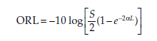
where S = backscattering capture coefficient, approximately
0.0015
for standard fiber at 1550 nm
L= fiber length, km
α= attenuation coefficient,
1/km
See calculation for ORL for SMF at 1550nm.
Assume fibre attenuation is 0.22 dB/km at 1550 nm,
S = 0.0015 with a nonreflective end.
L=20Km
After calculation using above generic values; ORL will come
as ~30 dB.
ITU-T G.959.1 recommends a minimum ORL of 24 dB for 2.5, 10, and 40 Gbps
fiber links.
A Bit error rate, BER, is a key parameter that
is used in assessing systems that transmit digital data from one location to
another.
BER can be influenced by a number of factors.
By manipulating the variables that can be controlled, it is possible to
optimize a system to provide the performance levels that are required. This is
normally undertaken in the design stages of a data transmission system so that
the performance parameters can be adjusted at the initial design concept
stages.
▪ Interference: The
interference levels present in a system are generally set by external factors
and cannot be changed by the system design. However, it is possible to set the
bandwidth of the system. By reducing the bandwidth, the level of interference
can be reduced. However, reducing the bandwidth limits the data throughput that
can be achieved.
▪ Increase transmitter power: It
is also possible to increase the power level of the system so that the power
per bit is increased. This has to be balanced against factors including the
interference levels to other users and the impact of increasing the power
output on the size of the power amplifier and overall power consumption and
battery life, etc.
▪ Lower order modulation: Lower
order modulation schemes can be used, but this is at the expense of data
throughput.
▪ Reduce bandwidth: Another
approach that can be adopted to reduce the bit error rate is to reduce the
bandwidth. Lower levels of noise will be received, and therefore the signal to
noise ratio will improve. Again, this results in a reduction of the data
throughput attainable.
It is necessary to balance all the available
factors to achieve a satisfactory bit error rate. Normally it is not possible
to achieve all the requirements, and some trade-offs are required. However,
even with a bit error rate below what is ideally required, further trade-offs
can be made in terms of the levels of error correction that are introduced into
the data being transmitted. Although more redundant data has to be sent with
higher levels of error correction, this can help mask the effects of any bit errors
that occur, thereby improving the overall bit error rate.
Definition 1:
The Q-factor, a function of the OSNR, provides a qualitative description
of the receiver performance. The Q-factor suggests the minimum signal-to-noise
ratio (SNR) required to obtain a specific BER for a given signal. OSNR is
measured in decibels. The higher the bit rate, the higher the OSNR ratio
required. For OC-192 transmissions, the OSNR should be at least 27 to 31 dB
compared to 18 to 21 dB for OC-48.
Definition 2:
The Quality factor is a measure of how noisy a pulse is for diagnostic
purposes. The eye pattern oscilloscope will typically generate a report that
shows what the Q factor number is. The Q factor is defined as shown in the
figure: the difference of the mean values of the two signal levels (level for a
“1” bit and level for a “0” bit) divided by the sum of the noise standard
deviations at the two signal levels. A larger number in the result means that
the pulse is relatively free from noise.
Definition 3:
Q is defined as follows: The ratio between the sums of the distance
from the decision point within the eye (D) to each edge of the eye, and the sum
of the RMS noise on each edge of the eye.
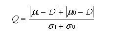
This definition can be derived from the following definition, which in
turn comes from ITU-T G.976 (ref. 3).
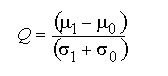
where m1,0 are the mean positions of each rail of the eye,
and s1,0 are the S.D., or RMS noise, present on each of these rails.
For an illustration of where these values lie within the eye see the
following figure:
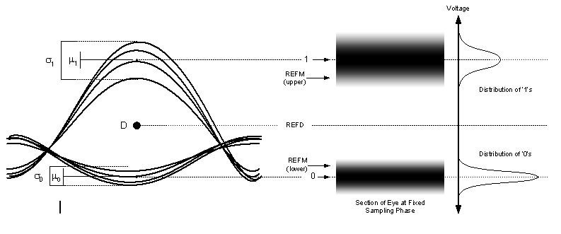
As Q is a ratio it is reported as a unit-less positive value
greater than 1 (Q>1). A Q of 1 represents complete closure of the received
optical eye. To give some idea of the associated raw BER a Q of 6 corresponds
to a raw BER of 10-9.
Q FACTOR AS DEFINED IN ITU-T G.976
The Q factor is the signal-to-noise ratio at the decision circuit in
voltage or current units, and is typically expressed by:
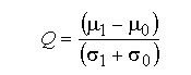 (A-1)
(A-1)
where µ1,0, is the mean value of the marks/space’s voltages or currents,
and s1,0 is the standard deviation.
The mathematic relations to BER when the threshold is set to the optimum
value are:
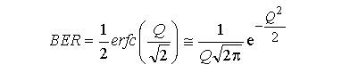 (A-2)
(A-2)
with:
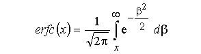 (A-3)
(A-3)
The Q factor can be written in terms of decibels rather than in linear
values:
![]() (A-4)
(A-4)
CALCULATION
OF Q-FACTOR FROM OSNR
The OSNR is the most important parameter that is associated with a given
optical signal. It is a measurable (practical) quantity for a given network,
and it can be calculated from the given system parameters. The following
sections show you how to calculate OSNR. This section discusses the
relationship of OSNR to the Q-factor.
The logarithmic value of Q (in dB) is related to the OSNR by
following Equation
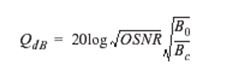
In the equation, B0 is the optical bandwidth of the end device
(photodetector) and Bc is the electrical bandwidth of the receiver filter.
Therefore, Q(dB)
is shown in
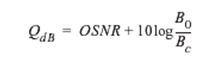
In other words, Q is somewhat proportional to the OSNR. Generally, noise
calculations are performed by optical spectrum analyzers (OSAs) or sampling
oscilloscopes, and these measurements are carried over a particular measuring
range of Bm. Typically, Bmis approximately 0.1 nm or 12.5 GHz for a given OSA.
From Equation showing Q in dB in terms of OSNR, it can be understood that if
B0 < Bc, then OSNR (dB )> Q (dB). For practical designs OSNR(dB)
> Q(dB), by at least 1–2 dB. Typically, while designing a high-bit rate
system, the margin at the receiver is approximately 2 dB, such that Q is about
2 dB smaller than OSNR (dB).
The Qfactor, is in fact a metric to identify the attenuation in the receiving
signal and determine a potential LOS and it-is an estimate of the
Optical-Signal-to-Noise-Ratio (OSNR) at the optical receiver. As
attenuation in the receiving signal increases, the dBQ value drops
and vice-versa. Hence a drop in the dBQ value can mean
that there is an increase in the Pre FEC BER, and a possible LOS could occur if
the problem is not corrected in time.
•
High Chromatic Dispersion (CD)
Robustness
•
Can avoid Dispersion Compensation Units (DCUs)
•
No need to have precise Fiber Characterization
•
Simpler Network Design
•
Latency improvement due to no DCUs
•
High Polarization Mode
Dispersion (PMD) Robustness
•
High Bit Rate Wavelengths deployable on all Fiber types
•
No need for “fancy”PMD Compensator devices
•
No need to have precise Fiber Characterization
•
Low Optical Signal-to-Noise
Ratio (OSNR) Needed
•
More capacity at greater
distances w/o OEO Regeneration
•
Possibility to launch lower
per-channel Power
•
Higher tolerance to Channels
Interferences
For Optical
communication to happen, a receiver (essentially a photodetector, either a PIN
or APD type) needs a minimum amount of power to distinguish the 0s and 1s from
the raw input optical signal.
The minimum
power requirement of the receiver is called the receiver sensitivity.
The optical
power at the receiver end has to be within the dynamic range of the receiver;
otherwise, it
damages the receiver (if it exceeds the maximum value) or the receiver cannot
differentiate
between 1s and 0s if the power level is less than the minimum value.
Signals lose strength as they are travel through the fiber:
this is known as attenuation.
Attenuation is measured in decibels (dB) with the relation:
![]()
where Pin and Pout refer to the optical power
going into and coming out of the fiber.
The attenuation of an optical fiber is
wavelength dependent. At the extremes of the transmission curve, multi-photon
absorption predominates. Attenuation is usually expressed in dB/km at a
specific wavelength. Typical values range from 10 dB/km for step-index fibers
at 850 nm to a few tenths of a dB/km for single-mode fibers at 1550 nm.
There are several causes of attenuation in an
optical fiber:
Rayleigh Scattering —
Microscopic-scale variations in the index of refraction of the core material
can cause considerable scatter in the beam, leading to substantial losses of
optical power. Rayleigh scattering is wavelength dependent and is less
significant at longer wavelengths. This is the most important loss mechanism in
modern optical fibers, generally accounting for up to 90 percent of any loss
that is experienced.
Absorption —
Current manufacturing methods have reduced absorption caused by impurities
(most notably water in the fiber) to very low levels. Within the bandpass of
transmission of the fiber, absorption losses are insignificant.
Bending —
Manufacturing methods can produce minute bends in the fiber geometry. Sometimes
these bends will be great enough to cause the light within the core to hit the
core/cladding interface at less than the critical angle so that light is lost
into the cladding material. This also can occur when the fiber is bent in a
tight radius (less than, say, a few centimeters). Bend sensitivity is usually
expressed in terms of dB/km loss for a particular bend radius and wavelength.
The buffer or
jacket on patch cords are often color coded to indicate the type of fiber used.
The strain relief "boot" that protects the fiber from bending at a connector
is color-coded to indicate the type of connection. Connectors made with a
plastic shell (such as SC
connectors) typically use a color coded shell. Standard
color coding's for jackets and boots (or connector shells) are shown below:
|
Buffer/jacket
color |
Meaning |
|
Yellow |
|
|
Orange |
|
|
Aqua |
10 gig laser-optimized
50/125 micrometer multi-mode optical fiber |
|
Grey |
outdated color code
for multi-mode optical fiber |
|
Blue |
Sometimes
used to designate polarization-maintaining optical fiber |
|
Connector
Boot |
Meaning |
Comment |
|
|
Blue |
Physical
Contact (PC), 0° |
mostly used
for single mode fibers; some manufacturers use this for polarization-maintaining optical
fiber. |
|
|
Green |
Angle
Polished (APC), 8° |
|
|
|
Black |
Physical
Contact (PC), 0° |
|
|
|
Grey, |
Beige |
Physical Contact (PC),
0° |
multimode fiber
connectors |
|
White |
Physical Contact (PC),
0° |
|
|
|
Red |
|
High
optical power. Sometimes used to connect external pump lasers or Raman pumps. |
|
CDC
allows operators to future proof their network, so they are able to optimize,
scale, and flexibly meet any future bandwidth demands.
▪ Directionless: for the ability to
route a wavelength across any viable path in the network
▪ Colorless: for the ability to receive any wavelength on any port.
▪Contentionless: eliminates wavelength
blocking, allowing the add/drop of a duplicate wavelength onto a single
mux/demux
▪ Flexible grid: for the ability to
future-proof the network for any higher capacity channel that needs >50GHz
spectrum
The CDC solution allows the operator to handle
unpredictable A-Z services or temporary bandwidth demands over the full life of
the network. Reconfigurations such as wavelength defragmentation and route
optimization are also made possible to scale the network for support of more
services. CDC also supports the transport of Super Channels when these become
available.
CDC can operate with a photonic control plane
for increased automation of operations as well as to support automated photonic
restoration and other future capabilities.
Gridless networks are the evolution of photonic
line systems to improve spectral efficiency and flexibilities
Channel grid is no longer required to be centered at ITU
wavelengths/frequencies.
▪ To get improved
spectral efficiency with existing 40G/100G technology.
▪ Define a
super-channel that has multiple sub-channels within it, in order to fit the
same channels in a smaller region of the spectrum.
▪ Support higher
line-rate transponders.
▪ In order to
get the same reach/performance from 400 Gb/s and 1 Tb/s transponders, we have
no choice but to increase the spectral width of these signals well beyond 50GHz
or even 100GHz spacing.
Definition of coherent light
A
coherent light consists of two light waves that:
1) Have
the same oscillation direction.
2) Have
the same oscillation frequency.
3) Have
the same phase or maintain a constant phase relationship with each other. Two
coherent light waves produce interference within the area where they meet.
Principles of Coherent Communication
Coherent
communication technologies mainly include coherent modulation and coherent
detection.
Coherent
modulation uses the signals that are propagated to change the frequencies,
phases, and amplitudes of optical carriers. (Intensity modulation only changes
the strength of light.)
Modulation
detection mixes the laser light generated by a local oscillator (LO) with the
incoming signal light using an optical hybrid to produce an IF signal that
maintains the constant frequency, phase, and amplitude relationships with the
signal light.
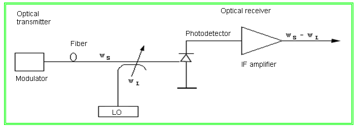
The two ideas behind using the coherent communication
techniques are:-
First, the receiver sensitivity can
be improved approximately by up to 20 dB compared with that of IM/DD systems.
Second, the use of coherent detection can allow a more efficient use of fiber
bandwidth by increasing the spectral efficiency of WDM systems.
As we know that both homodyne or heterodyne detection can be
used to convert the received optical signal into an electrical form. In case of homodyne detection, the optical
signal is demodulated directly to the baseband. Although simple in concept,
homodyne detection is difficult to implement in practice, as it requires a
local oscillator whose frequency matches the carrier frequency exactly and
whose phase is locked to the incoming signal. Such a demodulation scheme is
called synchronous and is essential for homodyne detection. Although optical
phase-locked loops have been developed for this purpose, their use is
complicated in practice.
Heterodyne detection simplifies the receiver design, as
neither optical phase locking nor frequency matching of the local oscillator is
required. However, the electrical signal oscillates rapidly at microwave
frequencies and must be demodulated from the IF band to the baseband using
techniques similar to those developed for microwave communication systems.
Demodulation can be carried out either synchronously or asynchronously.
Asynchronous demodulation is also called incoherent in the radio communication
literature. In the optical communication literature, the term coherent
detection is used in a wider sense.
A lightwave system is called coherent as long as it uses a
local oscillator irrespective of the demodulation technique used to convert the
IF signal to baseband frequencies.
* In case of homodyne coherent-detection technique,
the local-oscillator frequency is selected to coincide with the signal-carrier
frequency.
* In
the case of heterodyne detection, the local-oscillator frequency is chosen
to differ from the signal-carrier frequency.
Fiber splitters/couplers divide optical power from one common port to
two or more split ports and combine all-optical power from the split ports to
one common port (1 × N coupler). They operate across the entire band or bands
such as C, L, or O bands. The three-port 1 × 2 tap is a splitter commonly used
to access a small amount of signal power in a live fiber span for measurement
or OSA analysis. Splitters are referred to by their splitting ratio, which is
the power output of an individual split port divided by the total power output
of all split ports. Popular splitting ratios are shown in the Table below;
however, others are available. The equation below can be used to estimate the
splitter insertion loss for a typical split port. Excess splitter loss adds to
the port's power division loss and is lost signal power due to the splitter
properties. It typically varies between 0.1 to 2 dB, refer to manufacturer's
specifications for accurate values.
It should be noted that the
splitter function is symmetrical.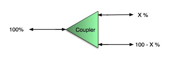
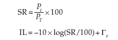
where IL
= splitter insertion loss for the split port, dB
Pi =
optical output power for single split port, mW
PT = total optical power
output for all split ports, mW
SR =
splitting ratio for the split port, %
Γe =
splitter excess loss (typical range 0.1 to 2 dB), dB
Common
splitter applications include
•
Permanent installation in a fiber link as a tap with 2%|98% splitting ratio.
This provides for access to live fiber signal power and OSA spectrum
measurement without affecting fiber traffic. Commonly installed in DWDM
amplifier systems.
• Video
and CATV networks to distribute signals.
•
Passive optical networks (PON).
• Fiber
protection systems.
Example
with calculation:
If a 0
dBm signal is launched into the common port of a 25% |75% splitter,
then the two split ports, output power will be −6.2 and −1.5 dBm. However, if a
0 dBm signal is launched into the 25% split port, then the common port output
power will be −6.2 dBm.
Calculation.
![]()
Launch
power=0 dB=1mW
Tap is 25%|75%
so
equivalent mW power which is linear will be
0.250mW|0.750mW
and
after converting them ,dBm value will be
-6.02dBm| -1.24dBm
Some of
the common split ratios and their equivalent Optical Power is available below
for reference.

The Optical Time Domain Reflectometer (OTDR) is useful for testing the
integrity of fiber optic cables. An optical time-domain
reflectometer (OTDR) is an opto-electronic instrument used to
characterize an optical fiber. An OTDR is the optical equivalent of an electronic time -domain reflectometer. It injects a series of optical pulses into the fiber under test. It
also extracts, from the same end of the fiber, light that is scattered (Rayleigh backscatter) or reflected back from points along the fiber. The
strength of the return pulses is measured and integrated as a function of time, and plotted as a function of fiber length.
Using an OTDR, we can:
1. Measure the distance to a fusion splice, mechanical splice,
connector, or significant bend in the fiber.
2. Measure the loss across a fusion splice, mechanical splice,
connector, or significant bend in the fiber.
3. Measure the intrinsic loss due to mode-field diameter variations
between two pieces of single-mode optical fiber connected by a splice or
connector.
4. Determine the relative amount of offset and bending loss at a splice
or connector joining two single-mode fibers.
5. Determine the physical offset at a splice or connector joining two
pieces of single-mode fiber, when bending loss is insignificant.
6. Measure the optical return loss of discrete components, such as
mechanical splices and connectors.
7. Measure the integrated return loss of a complete fiber-optic system.
8. Measure a fiber’s linearity, monitoring for such things as local
mode-field pinch-off.
9. Measure the fiber slope, or fiber attenuation (typically expressed in
dB/km).
10. Measure the link loss, or end-to-end loss of the fiber network.
11. Measure the relative numerical apertures of two fibers.
12. Make rudimentary measurements of a fiber’s chromatic dispersion.
13. Measure polarization mode dispersion.
14. Estimate the impact of reflections on transmitters and receivers in
a fiber-optic system.
15. Provide active monitoring on live fiber-optic systems.
16. Compare previously installed waveforms to current traces.
|
|
HD-FEC |
SD-FEC |
|
Definition |
Decoding
based on hard-bits(the output is quantized only to two levels) is called the
“HD(hard-decision) decoding”, where each bit is considered definitely one or
zero. |
Decoding based
on soft-bits(the output is quantized to more than two levels) is called the
“SD(soft-decision) decoding”, where not only one or zero decision but also
confidence information for the decision are provided. |
|
Application |
Generally,
for non-coherent detection optical systems, e.g., 10 Gbit/s, 40 Gbit/s,
also for some coherent detection optical systems with higher OSNR |
coherent
detection optical systems, e.g., 100 Gbit/s,400 Gbit/s. |
|
Electronics
Requirement |
ADC(Analogue-to-Digital
Converter) is not necessary in the receiver. |
ADC is
required in the receiver to provide soft information, e.g., coherent
detection optical systems. |
|
specification |
general
FEC per [ITU-T G.975];super FEC per [ITU-T G.975.1]. |
vendor
specific |
|
typical
scheme |
Concatenated
RS/BCH |
LDPC(Low
density parity check),TPC(Turbo product code) |
|
complexity |
medium |
high |
|
redundancy
ratio |
generally,
7% |
around
20% |
|
NCG |
about 5.6
dB for general FEC;>8.0 dB for super FEC. |
>10.0
dB |
|
Example(If
you asked your friend about traffic jam status on roads and he replies) |
maybe
fully jammed or free |
50-50
but I found other way free or less traffic |
Few analogies proving the subject:-
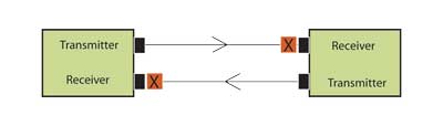
▪
If the distance is to short and
the attenuator is too close to the transmitter, the reflected light off the
attenuator will be directed back towards the Tx laser. Which will also blow
your transmitter.so we place it at Rx.
▪
Also keeping attenuator at Rx
will attenuate the noise along with the signal.
▪
The most important reason for
putting them on the RX side is that you are protecting that which needs to be
protected - the receiver in your optics. This way you know that you're not
going to potentially blow the receiver in your optics by plugging in too large
a signal because you assumed there was an attenuator on the TX at the far end,
and there wasn't.
▪
It's more convenient to test the
receiver power before and after attenuation or while adjusting it with your
power meter at the receiver, plus any reflectance will be attenuated on its
path back to the source.
Keynote on Using Attenuators with Fiber Optic Data Links
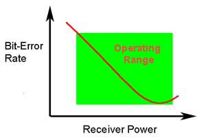
The ability of any fiber optic system to transmit data ultimately
depends on the optical power at the receiver as shown above, which shows the
data link bit error rate as a function of optical power at the receiver. (BER
is the inverse of signal-to-noise ratio, e.g. high BER means poor signal to
noise ratio.) Either too little or too much power will cause high bit
error rates.
Too much power, and the receiver amplifier saturates, too little and
noise becomes a problem as it interferes with the signal. This receiver power
depends on two basic factors: how much power is launched into the fiber by the
transmitter and how much is lost by attenuation in the optical fiber cable
plant that connects the transmitter and receiver.
If the power is too high as it often is in short single mode systems
with laser transmitters, you can reduce receiver power with an attenuator.
Attenuators can be made by introducing an end gap between two fibers (gap
loss), angular or lateral misalignment, poor fusion splicing (deliberately),
inserting a neutral density filter or even stressing the fiber (usually by a
serpentine holder or a mandrel wrap). Attenuators are available in models with
variable attenuation or with fixed values from a few dB to 20 dB or more.
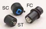
Gap-loss attenuators for multi mode
fiber
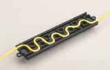
Serpentine attenuators for single mode
fiber
Generally, multimode systems do not need attenuators. Multimode sources,
even VCSELs, rarely have enough power output to saturate receivers. Single mode
systems, especially short links, often have too much power and need
attenuators.
For a single mode application, especially analog CATV systems, the most
important specification, after the correct loss value, is return loss or
reflectance! Many types of attenuators (especially gap loss types) suffer from
high reflectance, so they can adversely affect transmitters just like highly
reflective connectors.
Choose a type of attenuator with good reflectance specifications and
always install the attenuator ( X in the drawing) as shown at the
receiver end of the link. This is because it's more convenient to test the
receiver power before and after attenuation or while adjusting it with
your power meter at the receiver, plus any reflectance will be
attenuated on its path back to the source.
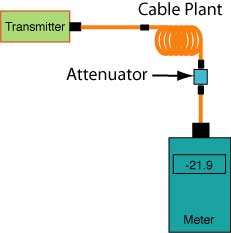
Test the system power with the transmitter turned on and the
attenuator installed at the receiver using a fiber optic power meter set to the
system operating wavelength. Check to see the power is within the specified
range for the receiver.
If the appropriate attenuator is not available, simply coil some patch
cord around a pencil while measuring power with your fiber optic power meter,
adding turns until the power is in the right range. Tape the coil and your
system should work. This type of attenuator has no reflectance and is very low
cost! The fiber/cable manufacturers may worry about the reliability of a cable
subjected to such a small bend radius. You should probably replace it with
another type of attenuator at some point, however.
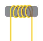
Single mode attenuator made by wrapping fiber or simplex
cable around a small mandrel. This will not work well with bend-insensitive fiber.
ref:http://www.thefoa.org/tech/ref/appln/attenuators.html
The first thing to note is that for each frame there are two sets of 20
parity bits. One set is associated with the end to end post FEC BER. The other
is used to measure the span by span raw BER. The points at which these parity
bits are terminated are illustrated below.
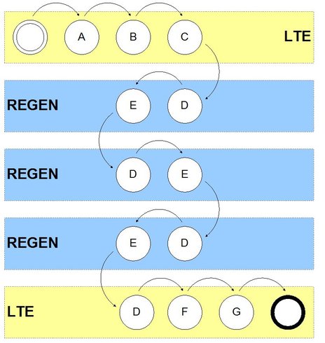
|
Processing point |
Process description |
|
A |
Calculate
and insert the post FEC parity bits (those over which FEC is calculated) over
the frame up to and including the MS OH. |
|
B |
Encode
FEC over the frame up to and including the MS OH. |
|
C |
Calculate
and insert the pre FEC parity bits (those over which FEC is not calculated) over the frame up to and
including the RS OH. |
|
D |
Terminate
the raw BER based on the pre FEC parity bits. |
|
E |
Re-calculate
the pre FEC parity bits over the frame up to, and including, the RS OH. |
|
F |
Decode
FEC to produce the final data. |
|
G |
Terminate
the post FEC BER based on the post FEC parity bits. |
We can use the raw BER extracted at each RS terminating point (regens
and LTEs) to estimate the post FEC BER. Note that this estimate is based on an
assumption of a Poisson distribution of errors. In contrast the real post FEC
BER can only be extracted at the MS terminating equipment (LTEs), and this is
used to feed into the PM error counts.
Following are the terminologies you will come across when referring FEC
Performance parameters:
PRE-FEC BER are the bit errors caused by attenuation, ageing, temperature
changes of the optical fiber. PRE-FEC indicates that the signal on the
optical fiber is FEC
encoded. The FEC decoder will recover the original signal, but
depending on the PRE_FEC BER it will succeed to recover the original
signal completely without errors.
Or, if the BER on the fiber is too high, the recovered signal will
contain bit errors.
If the signal was FEC encoded the remaining bit errors after
the decoder are called POST FEC BER.
The NO FEC BER are the bit errors detected when no FEC coding
is used on the optical fiber.
Uncorrected words are the word that FEC is not able to corrects. It
shows that the current FEC is not able to correct anymore and we need to look
for more advance FEC.
he optical link design essentially is putting the various optical
components, which we discussed earlier, so that information can be transmitted
satisfactorily. The satisfactoriness of the transmission can be defined in
terms of some characteristic parameters.
The user generally specifies the distance over which the
information is to be sent and the data rate to be transmitted. The Designer
then has to find the specification of the system components.
The designer generally has to define some additional criteria either as
per the standards or as per the user specifications.
The
Design criteria are given in the following.
Primary
Design Criteria
◦
Data Rate
◦
Link
length
Additional
Design Parameters
▪
Modulation format e.g.
Analog/digital
◦
Depends upon the type of signals
user want to transmit. For example, if it is a TV signal, then may be analog
transmission is more suited as it requires less bandwidth and better linearity.
On the other hand, if data or sampled voice is to be transmitted, digital
format may be more appropriate.
◦
The digital signals have to be
further coded to suite the transmission medium and for error correction.
▪
System
fidelity: BER, SNR
◦
The system fidelity defines the
correctness of the data received at the receiver.
◦
For digital transmission
it is measured by the Bit Error Ratio (BER) . The BER is defined as:-
◦
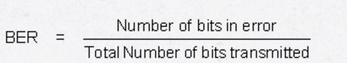
◦
In optical system, the BER has
to be less than 10E-9
◦
For analog system, the quality
parameter is the Signal-to-noise (SNR) ratio. In addition, there is a parameter
called the inter-modulation distortion, which describes the linearity of the
system.
▪
Cost :
Components, installation, maintenance
◦
Cost is one of the important
issues of the link design.
◦
The cost has three components,
components, installation and maintenance.
◦
The component and the
installations cost are the initial costs. Generally, the installation cost is
much higher than the component cost for long links. This is especially true for
laying the optical cable. It is therefore appropriate to lay the cables keeping
in view the future needs.
◦
The optical link is supposed is
supposed to work for at least 25years. The maintenance costs are as important
as the initial cost. An initial cheaper system might end up into higher
expenses in maintenance and therefore turn out to be more expensive as a whole.
▪
Upgradeability
◦
The optical fiber technology is
changing very rapidly and the data rates are increasing steadily.
◦
The system should be able to
adopt new technology, as well should be able to accommodate higher data rates
with least possible changes.
▪
Commercial
availability
◦
Depending upon which part of the
world one is, the availability of the components and the systems may be an
issue.
ref:http://nptel.ac.in/courses/117101054/16
Compared
with requirements for EDFAs for terrestrial applications and for Submarine
applications, there are major important differences making the two types of
amplifiers definitely two different components.
|
Terrestrial(Land)
system |
Submarine
System |
|
•Reliability of land-based equipment is somewhat relaxed,
corresponding to a 15-year required
lifetime. |
• Submarine systems are designed for a 25-year lifetime and a minimum
of ship repair that imply reliability and redundancy of all the critical components. |
|
• Terrestrial equipment should enable operation over a wide
temperature range of −5, +70°C (and −40, +85°C in storage conditions). This wide temperature range makes it necessary to implement
cooling means for the highest
temperatures and compensation means for temperature-sensitive devices. |
• In submarine amplifiers, heat is dissipated from the outer side of
the repeater container into the sea. Such a container is designed in order to
make the heat go through the box from the pump device to the outer side,
ensuring moderate temperature in all points. Temperature of the deep sea is
indeed around +5°C. Specific care is taken for repeaters located at the coast
or in shallow water, in order to guarantee no pump failure while avoiding
Peltier cooling. For reliability reasons, no glue is used on the optical path. The
constant temperature of the devices and the doped fiber incorporated in the
amplifier makes it possible to perfectly tailor the gain spectrum of the
submerged EDFAs, owing to very accurate equalizing filters and to
concatenating hundreds of amplifiers. This would not be possible for land-based amplifiers whose gain cannot
be guaranteed below 1 dB for a 30-nm bandwidth partly due to such temperature
changes (while a few tenths of dB of gain excursion is reached for submarine
amplifiers). |
|
• The infrastructure itself of terrestrial systems determines the
actual characteristics of the amplifier that needs to cope with important
variations of the span loss between two amplifier sites. In addition, for
economic reasons, the amplifiers cannot be tailored to cope with this
nonuniform link. |
• In submarine systems, the link is manufactured at the same time as
the amplifiers and much attention is paid to guarantee constant attenuation
loss between amplifier values, while the amplifier has been designed to
perfectly adapt to the link characteristics. |
|
• There are high gain range (20 to 35 dB) of the amplifiers
incorporated in land-based systems and allowed by the margins given on the
OSNR due to the reduced total link length. Gain equalizers therefore compensate for much larger gain excursion
values than in submarine amplifiers and should therefore be located at
amplifier midstage in order not to impact their equalizing loss on the
amplifier output power. |
• On the contrary, such filters can be placed after the single section
of doped fiber that composes the amplifier in the case of submarine
applications. |
The Bit Error Rate (BER) of a digital optical
receiver indicates the probability of an incorrect bit identification. In other
words, the BER is the ratio of bits received in error to the total number of
bits received. Below lists different values for BER and their corresponding
errors per bits and over time.
As we know that, the photocurrent is converted to a voltage then
measured. The measurement procedure involves a decision as to whether the bit
received is a 1 or a 0. The BER is not only a function of the noise in the
receiver and distortion in the system but also on the decision level voltage
that is the threshold level above which the signal is classified as a 1 and
below which the signal is classified as a 0. Even an ideal signal with no noise
nor distortions has a non-zero BER if the decision level is set too high or too
low. For example, if VD is set above the voltage of the 1 bit, the BER is 0.5,
assuming equal probability of receiving a one and a zero.
|
BER |
Error per 10E-15 bits |
@
10Gbps, One error in |
|
1x10⁻⁶ |
10,00,00,000 |
0.1
msec |
|
1x10⁻⁹ |
1,00,000 |
0.1
sec |
|
1x10-12 |
100 |
1.7
min |
|
1x10-15 |
1 |
1.2
days |
Mathematically, the Bit Error
Rate is expressed as
BER =
p(1)P(0 ⁄ 1) +
p(0)P(1 ⁄ 0)
where
p(1) and p(0) are the probabilities of receiving a 1 and a 0, respectively.
P(0/1) is the probability of deciding a 0 when the bit is actually a 1, and
P(1/0) is the probability of deciding a 1 when the bit is a 0.
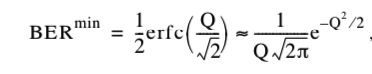
Minimum BER as a function of Q
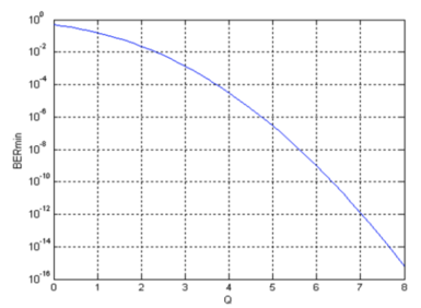
Noise sources can be categorised as
an active and passive.
Active sources such as optical plugs,lasers,
receivers, and amplifiers generate noise in the fiber link.
Passive sources such as connectors, fiber,
splices, and WDMs cause interference by distorting or reflecting the
propagating signal power.
Below are ten major noise sources:
1. Signal-spontaneous
noise (si-sp): This type of noise is generated by the
signal mixing with amplified spontaneous emission noise generated in an optical
amplifier. It is typically the dominant noise source in an amplified optical
link. It is also known as amplified spontaneous emissions (ASE) noise.
2. Spontaneous-spontaneous
noise (sp-sp): This type of noise is generated by ASE
mixing with itself.
3. Shot
noise (sh): This kind of electrical noise is generated by
the receiver photodiode in both PIN and APD type receivers. APD type receivers
have a better signal to noise ratio (SNR) due to their internal multiplication
gain mechanism. Receiver noise level and minimum OSNR are established in
transceiver design and cannot be controlled by system planning other than by
selecting better transceivers.
4. Shot-spontaneous
noise (sh-sp): This kind of noise is generated by shot
noise added along-with ASE noise in the receiver. It is accounted for the
transceiver's OSNR specifications.
5. Thermal
noise (th): This type of noise is generated by the front
end of the receiver diode due to thermal activity and is accounted for in the
transceiver's OSNR specifications. The RMS photodiode
6. Multiple
path interference noise (MPI): This noise is generated by
the signal reflecting multiple times in the fiber and interfering with itself.
Reflections are due to Rayleigh scattering and other reflective events such as
connectors and splices. It is typically a concern for high signal powers and in
distributed Raman amplifiers with high gains. This noise source is also known
as double Rayleigh scattering (DRS). To keep MPI noise to a minimum, use
good-quality, and clean ultra-polish (UPC) or angle polish (AP) type fiber
connectors. Fiber splices that show OTDR reflections should be re-spliced.
7. Source
spontaneous emissions (SSE): This noise is due to
spontaneous photon emissions during the lasing process. These random photons
add to the laser's amplitude and phase, causing noise.
8. Mode
partition noise (MPN): This noise occurs because of random
variations of individual laser modes even though the total laser output power
remains constant. The noise is generated in fibers where the signal dispersion
wavelength is not zero. The fluctuating modes travel at different group
velocities due to chromatic dispersion, which results in mode desynchronization
and adds receiver noise. MPN occurs for MLM lasers but can also occur for SLM
lasers that have significantly large side nodes and where the side mode
suppression ratio (SMSR) is less than 20 dB.
9. Cross
talk noise: DWDM (dense wavelength-division multiplexing)
can cause interference noise as channel cross talk. The signal from one WDM
channel appears on another channel resulting in interference. This is because a
WDM cannot provide total 100% channel isolation. Typical adjacent channel
isolation is approximately 30 dB down from adjacent channel signal power. At
this level, the interference is not significant in most systems. However, it
can be a concern for high channel launch powers.
10. Nonlinear distortions: Fiber can also cause
noise interference when high power signals interact with the fiber, resulting
in nonlinear distortions such as four-wave mixing. Maintaining low signal power
below recommended limits can help keep this interference to a minimal level.
The optical
spectrum analyzer (OSA) is the device typically used to measure OSNR. Signal
and noise measurements are made over a specific spectral bandwidth Br , which
is referred to as the OSA's resolution bandwidth (RBW). The RBW filter acts as
a bandpass filter allowing only the set amount of light spectrum to strike the
OSA's photodetector. The photodetector measures the average optical power in
the spectral width. It cannot discriminate between two separate signals in the
RBW spectrum. If there is more than one signal in RBW, it will treat and
display them as one. Therefore, the ability of an OSA to display two closely
spaced signals as two distinct signals is determined by the RBW setting.
Typically, an OSA's RBW range is adjustable between 10 and 0.01 nm with common
settings of 1.0, 0.5, 0.1, and 0.05 nm.
Noise power on
signal cannot be measured directly
because it is overpowered by the signal itself. Therefore, the noise
measurement is performed at both sides of the signal, i.e outside of the signal
boundary, using the OSA's noise equivalent bandwidth (NEB) filter. The results
are then interpolated to determine the noise power at the signal wavelength.
The NEB filter has a rectangular passband and provides a more accurate noise
measurement than the standard RBW filter.
The BER test needs to be
ran till enough bits gets transmitted and results are statistically usable. Actually,
the test is run for an infinite amount of time, transmitting an infinite number
of bits, that results in the channel's true BER. However, this is not
practical, and thus a statistical method is used to determine the channel's BER
to a certain confidence level of factor. This confidence level is a measure of
percentage which represents the probability the true BER is equal to or better
than the test BER. Typical confidence levels are 95% or 99%.
For a given
design at a BER (such as 10-12 and a line rate of OC-3, or 155 Mbps), the
network would have one error in approximately ten days. It would take thousand
days to record a steady-state BER value. e.g. to provide a BER of 1e−12, there
can be a one-bit error per 1e12 bits. At a 1.25 Gbps bit rate, it will take
around 800 seconds (13.3 minutes) to transmit/receive 1e12 bits. Therefore,
measurements sufficient to ascertain the BER down to 1e−12 or lower (at a
sufficient confidence level) will generally require transmission a greater
number of bits than 1e12 bits. Computer simulations on a system model can also
be performed to determine BER. However, computer simulations presently can
typically run about 1e6 bits in about an hour. Many existing applications
require BER performance that is down to a level of 1e−12 or lower (e.g.,
1e−17). Therefore, measurements or computer simulations might impose
unacceptable time constraints.
This is why
BER calculations are quite difficult. On the other hand, Q-factor analysis is
comparatively easy. Q is often measured in dB. The next question is how to
calculate Q dynamically. This is done from OSNR.
In other
words, Q is somewhat proportional to the OSNR. Generally, noise calculations
are performed by optical spectrum analyzers (OSAs) or sampling oscilloscopes,
and these measurements are carried over a particular measuring range of Bm.
Typically, Bm is approximately 0.1 nm or 12.5 GHz for a given OSA. From
equation, showing Q in dB in
terms of OSNR,
it can be understood that if B0 < Bc, then OSNR (dB )> Q (dB). For
practical designs OSNR(dB) > Q(dB), by at least 1–2 dB. Typically, while
designing a high bitrate system, the margin at the receiver is approximately 2
dB, such that Q is about 2 dB smaller than OSNR (dB).
Traditional
DWDM network was static network. In earlier DWDM networks, it was point to
point or rings (with point to point). Every channel route was pre-defined. To
add and drop any new channel, a lot of manual intervention required.
ROADM is
Reconfigurable (also some vendor refers remotely reconfigurable) OADM where,
reconfigurability is a very desirable attribute in an OADM. Reconfigurability
refers to the ability to select the desired wavelengths to be dropped and added
on the fly, as opposed to having to plan ahead and deploy appropriate
equipment. This allows carriers to be flexible when planning their network and
allows lightpaths to be set up and taken down dynamically as needed in the
network.
A
reconfigurable optical add/drop multiplexer (ROADM) can provide flexibility and
reconfigurability for an optical transport network (OTN). Such capabilities
enable network operators to quickly and flexibly respond to network changes,
such as establishing new light paths or releasing existing light paths.
ROADM
application scenarios include colored & directioned, colored &
directionless, and colorless & directionless.
The signal transmission
quality is not stable over a long period of time because of the polarization
effects occurring along the propagation path. The Time-varying system
performance (TVSP) is deduced from testbed experiments where the fluctuations
of the Q-factor are measured over a prolonged period of time. From this measurement,
a Gaussian distribution is fitted to the measurements in order to deduce the
standard deviation (s) and the average (mean Q) of the Q-factor distribution.
The following effects are the main sources of
Q-factor fluctuations:
PDL(polarization-dependent loss):
This corresponds to the dependence of the
insertion loss of passive components to the signal state of polarization
(SOP).
PHB (polarization hole burning):
This corresponds to the dependence of the
optical amplifier gain to the signal SOP. The PHB is an effect that is
significant in single-wavelength transmission since the degree of polarization
(DOP) of a laser source is close to 100% unless a polarization scrambler is
used. In WDM transmission systems, including a large number of wavelengths,
however, the DOP of the optical stream is close to 0% due to the random
distribution of the different wavelengths SOP. This effect becomes, therefore,
negligible in a WDM transmission system.
PDG
(polarization-dependent gain):
This corresponds to the dependence of the EDFA
gain to the pump SOP. The PDG can be considered for EDFA as equivalent to the
PDL for passive components, and the impact on the transmission quality is the
same as the PDL.
PMD(polarization mode dispersion):
This corresponds to the dependence of the fiber
refractive index on the signal SOP.
SE is
defined as the information capacity of a single channel (in bit/s) divided by
the frequency spacing Δf (in Hz) between the carriers of the WDM comb:
SE
= Rs log2(M) /Δf (1+r)
where Rs is the symbol rate, M is the number of constellation
points of the modulation format, and r is the redundancy of the forward error
correction (FEC) code, for example, r = 0.07 for an FEC with overhead (OH)
equal to 7%
More the SE, more data can be transmitted in a fiber. The total
system capacity (defined as the maximum information in bit/s that can be
transmitted by the WDM comb) is obtained as the product between the SE and the
available bandwidth. The maximization of the SE thus plays an important role in
the maximization of the overall system capacity.
The total system capacity (defined as the maximum information in
bit/s that can be transmitted by the WDM comb) is obtained as the product
between the SE and the available bandwidth. The maximization of the SE thus
plays an important role in the maximization of the overall system capacity.
In the past
years, the SE of optical systems has significantly increased, mainly due to the
advent of coherent-detection technologies, which enabled the use of high-order
modulation formats based on polarization-division multiplexing (PDM) [2], such
as PDM-QPSK (quadrature phase-shift keying), with M = 4, PDM-16QAM
(quadrature-amplitude modulation), with M = 8, and PDM-64QAM, with M = 12.
However, the use of high-order modulation formats requires a higher optical
signal-to-noise ratio (OSNR), which may result in a significantly reduced
achievable transmission distance.
To
increase the SE, and consequently, the overall system capacity, involves
reducing the frequency spacing Δf between the WDM sub-carriers. Here normalized
frequency spacing 𝛿f
and symbol Rate Rs defined as
𝛿f =Δf /Rs
For ultimate spectral efficiency, WDM channel
spacings are reduced until the optical spectra of neighboring channels start to
overlap noticeably. But this imposes linear crosstalk between adjacent WDM
channels and becomes a main source of degradation. An efficient countermeasure
to limit the crosstalk is based on an accurate spectral shaping of each
sub-channel of the WDM comb is known as "Nyquist-WDM,"
Where the transmission of PDM-QPSK WDM signals
with channel spacing equal to the symbol rate
The technique has also been successfully
applied to the generation and transmission of higher-order modulation formats,
such as PDM-8QAM, PDM-16QAM, PDM-32QAM, and PDM-64QAM with frequency spacing
values equal or very close to the symbol rate.
Depending on the normalized frequency spacing 𝛿f among the
WDM channels, three different categories of Nyquist-WDM signaling, which
are
• 𝛿f = 1
(i.e., Δf = Rs): Ideal Nyquist-WDM
• 𝛿f > 1
(i.e., Δf > Rs): Quasi-Nyquist-WDM
• 𝛿f < 1
(i.e., Δf < Rs): Super-Nyquist-WDM
The main
purposes of coherent detection are
(i) to linearly recover the In-Phase (I) and
Quadrature (Q) components of the incoming signal, and
(ii) to
suppress or cancel the common mode noise.
This is
because of the reduction of the minimal distance between two points of the
constellation, which reduces the resilience to channel impairments. For
instance, going from a PDM-QPSK up to a PDM-16QAM transmission doubles the data
rate at the cost of an optical reach divided by a factor of 5.
Key
characteristics of optical amplifiers are gain, gain bandwidth, gain
efficiency, noise, gain saturation, and
polarisation sensitivity:
• Gain is defined the ratio of output power to
input power (measured in decibels).
• Gain efficiency is defined as the gain as a
function of input power (decibels per milliwatt).
• Bandwidth is a function of frequency, and as
such, gain bandwidth is the range of frequencies over which the amplifier is
effective.
•
Gain saturation is the maximum output power of the amplifier, beyond which it
cannot increase despite the input power increase.
• Noise is an inherent characteristic of
amplifiers. In optical amplifiers, noise is due to the spontaneous emission of
excited ions.
• Polarization sensitivity is the gain
dependence of optical amplifiers on the polarization of the signal.
Main issues associated with EDFA designs are as follows:
1. The first issue is the flat gain. As EDFAs do not amplify all
wavelengths through them the same; thus, the gain is not exactly flat.
2. The second issue is the pump power-sharing. The pump power is
shared by all wavelengths in the link. Therefore the more the wavelengths, the lesser power
per wavelength will be available. However, as wavelengths can get drop but not
added, or some wavelengths get lost due to failures, EDFAs will amplify few
wavelengths more.
These two issues can be mitigated by properly engineering the
WDM system and by dynamic gain control.
3. The
third issue is not as simple and is addressed differently. When engineering
a fiber-optic path, it should be
remembered that optical noise sources are cumulative and that the ASE of EDFAs
introduces noise that degrades the signal to noise ratio (SIN). Although a
strong optical signal launched into the fiber could overcome this, near the
zero-dispersion wavelength region, four-wave mixing would become dominant, and
it would degrade the SIN ratio.
Following are the major parameters associated
with fibers:
•
Forward attenuation/km
•
Backward attenuation/km (if asymmetric)
•
Polarization mode dispersion
•
Polarization-dependent loss (PDL)
•
Dispersion (chromatic and material)
•
Zero-dispersion wavelength
•
Dispersion flatness over spectrum range
•
Birefringence
•
Cutoff wavelength.
Following are the major parameters associated
with optical light sources:
•
OCh output power
•
OCh wavelength AQ
•
Line spacing
•
Cutoff A (tunable sources)
•
Tunability speed (tunable sources)
•
Spectral width (tunable sources)
•
Line width (light sources)
•
Modulation depth (modulated sources) • Bit rate
(max-min) (modulated sources) •
•
Source noise
•
Dependency on bias
Following are the major parameters associated
with optical light receivers:-
•
Minimum threshold optical power, minimum
sensitivity
•
Responsiveness per wavelength, AQ
•
Wavelength discrimination
•
Receiver bit rate (max-min)
•
Min-max threshold level (one-zero)
•
Dependency
on one’s density
•
Dependence
on polarization
•
Demodulation
•
Receiver
noise
•
Dependency
on bias
•
Dependency
on temperature
The temperature sensitivity of an erbium-doped
fiber amplifier (EDFA) is approximately –0.023 dB/°C in the
temperature range of 25 to 95°C.
The gain of an EDFA often
falls as the temperature increases. Temperature sensitivity is generally due to
the misalignments of the fi- ber couplers that are inherent to the design, but
slight effects from absorption and changes in the indices of refractions may
also contribute.
Reference :
C. Liu et al.
“Temperature and Electromagnetic Effects on Erbium-Doped Fiber Amplifier
Systems,” Optical Engineering, 37(7), pp. 2095–2100, July 1998.
1. increasing the signal’s frequency;
2.
increasing the number of fibers;
3.
increasing the number of channels;
4.
increasing the modulation complexity.
The first option would
require a proportional increase in bandwidth, while the other options would
require the inclusion or replacement of equipment, resulting in higher cost,
complexity, and power consumption.
The quality of the transmitted signal can be
analyzed at a glance through an eye diagram, .which is generated by
superimposing repetitive samples of the PAM2 signal. The vertical eye-opening
is related to the signal amplitude and signal-to-noise ratio (SNR). Higher the
opening, better the SNR.
An OTDR is a
test instrument that sends short light pulses down an optical fiber to
determine the fiber's characteristics, attenuation, and length. Testing needs
OTDR at one end of the fiber for the test. At the other end of the fiber a good
reflective fiber end is required, such as an open connector, to produce strong
reflections for good readings,
OTDR launches
short pulses into the fiber over three or four wavelengths (typically 1310,
1410, 1550, and 1625 nm) and measures the elapsed time between the reflected
pulses
The total
elapsed time measured for the reflected pulses must be divided by two in order
to account for the light pulse traveling twice the fiber length. The fiber
length is determined by the OTDR from the pulse delay.
Power values
w.r.t Intensity and Distance graph is plotted, which gives information about
the losses, reflection, splice, break etc.OTDR traces can help locate
high-reflective events for repair.ORL can be measured with an ORL test set or
an OTDR
If the end of
the fiber provides a poor reflection such as with an angle connector or broken
fiber, the fiber length is too long, or the loss is too high, then measurements
using this method may not be possible.
As we know that to improve correction capability, more
powerful and complex FEC codes must be used. However, the more complex the FEC
codes are, the more time FEC decoding will take. This
term "baud" originates from the French engineer Emile Baudot, who was
the inventor of 5-bit teletype code. The Baud rate actually refers to the
number of signal or symbol changes that occurs per second. A symbol is one of
the several voltage, frequency, or phase changes.
Baudrate =
bitrate/number of bits per symbol ;
signal
bandwidth = baud rate;
Baud rate:
It is the rate symbols which are generated at
the source and, to a first approximation, equals to the electronic bandwidth of
the transmission system. The baud rate is an important technology-dependent
system performance parameter. This parameter defines the optical bandwidth of
the transceiver, and it specifies the minimum slot width required for the
corresponding flow(s).
Baud rate/symbol rate/transmission rate for a
physical layer protocol is the maximum possible number of times a signal can
change its state from a logical 1 to logical 0 or or vice-versa per second.
These states are usually voltage, frequency, optical intensity or phase. This
can also be described as the number of symbols that can be transmitted in 1
second. The relationship between baud rate and bitrate is given as.
Bit rate =
baud rate * number of bits / baud
The number of bits per baud is deduced from the
existing modulation scheme. Here, we are assuming that the number of bits per
baud is one, so, the baud rate is the exactly same as the bit rate.
The spectral-width of the wavelength in GHz is
equal to the symbol rate in Gbaud measured at the 3 dB point or the point where
the power is half of the peak. As the baud rate increases, the spectral-width
of the channels will increases proportionally. The higher baud rates,
therefore, are unable to increase spectral efficiency, though there can be
exceptions to this rule where a higher baud rate better aligns with the
available spectrum. Increasing wavelength capacity with the baud rate, has far
less impact on reach than increasing it with higher-order modulation.
Higher baud rates, offer the best potential for
reducing the cost per bit in Flexi-grid DWDM networks and also in
point-to-point fixed grid networks, even though higher baud rates are not
significant in 50 GHz fixed grid ROADM networks. Higher baud rates also
requires all the components of the optical interface, including the DSP,
photodetector and A/D converters and modulators, to support the higher
bandwidth. This places a limit on the maximum baud rate that is achievable with
a given set of technology and may increase the cost of the interfaces if more
expensive components are required.
dBm or decibel-milliwatt is an electrical power
unit in decibel
(dB), referenced to one milliwatt (mW).
The power in decibel-milliwatts (P(dBm)) is
equal to 10 times base 10 logarithm of the power in milliwatts (P(mW)):
P(dBm) = 10
· log10( P(mW) / 1mW )
The power in milliwatts (P(mW)) is equal to 1mW
times 10 raised by the power in decibel-milliwatts (P(dBm)) divided by 10:
P(mW) = 1mW
· 10(P(dBm) / 10)
1 milliwatt is equal to 0 dBm:
1mW = 0dBm
1 watt is equal to 30dBm:
1W = 1000mW = 30dBm
How to convert mW to dBm
How to convert optical power in milliwatts(mW)
to dBm.
The power in dBm is equal to the base10
logarithm of the power in milliwatts(mW):
P(dBm) = 10
· log10( P(mW) / 1mW )
For example: what is the power in dBm for power
consumption of 100mW?
Solution:
P(dBm) = 10
· log10( 100mW / 1mW ) = 20dBm
How to convert dBm to mW
How to convert power in dBm to milliwatts (mW).
The power in milliwatts (P(mW)) is equal to 10
raised by the power in dBm (P(dBm)) divided by 10?
P(mW) = 1mW
· 10(P(dBm) / 10)
For example: what is the power in milliwatts
for power consumption of 20dBm?
Solution:
P(mW) = 1mW
· 10(20dBm / 10) = 100mW
How to Convert Watt to dBm
How to convert power in watts (W) to dBm.
The power in dBm is equal to the base 10
logarithm of the power in watts (W) plus 30dB:
P(dBm) = 10
· log10( P(W) / 1W ) + 30
For example: what is the power in dBm for power
consumption of 100W?
Solution:
P(dBm) = 10
· log10( 100W / 1W ) + 30 = 50dBm
How to convert dBm to Watt
How to convert power in dBm to watts (W).
The power in watts (P(W)) is equal to 10 raised
by the power in dBm (P(dBm)) minus 30dB divided by 10:
P(W) = 1W ·
10( (P(dBm) - 30) / 10)
For example: what is the power in watts for
power consumption of 40dBm?
Solution:
P(W) = 1W ·
10( (40dBm - 30) / 10) = 10W
How to convert dBW to dBm
How to convert power in dBW to dBm.
The power in dBm is equal to the base 10
logarithm of the power in watts (W):
P(dBm) =
P(dBW) + 30
For example: what is the power in dBm for power
consumption of 20dBW?
Solution:
P(dBm) =
20dBW + 30 = 50dBm
How to convert dBm to dBW
How to convert power in dBm to dBW.
The power in dBW (P(dBW)) is equal to 10 raised
by the power in dBm (P(dBm)) divided by 10:
P(dBW) =
P(dBm) - 30
For example: what is the power in watts for
power consumption of 40dBm?
Solution:
P(dBW) =
40dBm - 30 = 10dBW
dBm to Watt, mW, dBW conversion table
|
Power (dBm) |
Power (dBW) |
Power (watt) |
Power (mW) |
|
-100 dBm |
-130 dBW |
0.1 pW |
0.0000000001 mW |
|
-90 dBm |
-120 dBW |
1 pW |
0.000000001 mW |
|
-80 dBm |
-110 dBW |
10 pW |
0.00000001 mW |
|
-70 dBm |
-100 dBW |
100 pW |
0.0000001 mW |
|
-60 dBm |
-90 dBW |
1 nW |
0.000001 mW |
|
-50 dBm |
-80 dBW |
10 nW |
0.00001 mW |
|
-40 dBm |
-70 dBW |
100 nW |
0.0001 mW |
|
-30 dBm |
-60 dBW |
1 μW |
0.001 mW |
|
-20 dBm |
-50 dBW |
10 μW |
0.01 mW |
|
-10 dBm |
-40 dBW |
100 μW |
0.1 mW |
|
-1 dBm |
-31 dBW |
794 μW |
0.794 mW |
|
0 dBm |
-30 dBW |
1.000 mW |
1.000 mW |
|
1 dBm |
-29 dBW |
1.259 mW |
1.259 mW |
|
10 dBm |
-20 dBW |
10 mW |
10 mW |
|
20 dBm |
-10 dBW |
100 mW |
100 mW |
|
30 dBm |
0 dBW |
1 W |
1000 mW |
|
40 dBm |
10 dBW |
10 W |
10000 mW |
|
50 dBm |
20 dBW |
100 W |
100000 mW |
|
60 dBm |
30 dBW |
1 kW |
1000000 mW |
|
70 dBm |
40 dBW |
10 kW |
10000000 mW |
|
80 dBm |
50 dBW |
100 kW |
100000000 mW |
|
90 dBm |
60 dBW |
1 MW |
1000000000 mW |
|
100 dBm |
70 dBW |
10 MW |
10000000000 mW |
Wavelength
Selective Switches or WSS form the heart of ROADM. A WSS route wavelength
channels between input port (s) to the output port(s), whereby the state of
connectivity of the switch can be set on a wavelength by wavelength basis. WSS
Modules are available in switch sizes ranging from 1x2 to 1x9, with some recent
product announcements extending this to 1x20 to 1x23.
WSS Technologies:
1. MEMS
2. DLP (Digital Light Processing)
3. Liquid Crystals (LC) Cells
4. Liquid Crystals on Silicon (LCoS)
5. Hybrid ( LC+MEMS)
REFERENCES
1.
Lightwave Technology Telecommunication Systems by
Govind P. Agrawal
2.
Undersea Fiber Communication Systems by Jose ́
Chesnoy
3.
Fault Detectability in Dwdm By Stamatios V.
Kartalopoulos
4.
Enabling Technologies for High
Spectral-Efficiency Coherent Optical Communication Networks by Xiang Zhou
Chongjin Xie
5.
Multiple Internet Resources
6.
www.mapyourtech.com (my website)
ABOUT THE AUTHOR
Sanjay
Yadav, is an enthusiastic Optical Fiber Communication Professional having
experience in various optical industries dealing with products, services
,design and operations. He believes in sharing knowledge which can help young
enthusiasts to grow in their professional career.
You can
visit his work on www.mapyourtech.com and reach
on feedback@mapyourtech.com