
Red and Blue Bands in DWDM: Complete Technical Guide
Understanding Wavelength Band Division, EDFA Gain Characteristics, and Cost-Effective System Design in Dense Wavelength Division Multiplexing Networks
Introduction
Dense Wavelength Division Multiplexing (DWDM) represents a fundamental breakthrough in optical networking, enabling multiple optical signals to traverse a single fiber simultaneously through precise wavelength separation. Within the ITU-approved DWDM spectrum, the concepts of "red band" and "blue band" serve as critical design parameters that directly influence system cost, amplification efficiency, and network scalability. These designations, rooted in electromagnetic spectrum conventions from physics and astronomy, have profound practical implications for network architects and optical engineers.
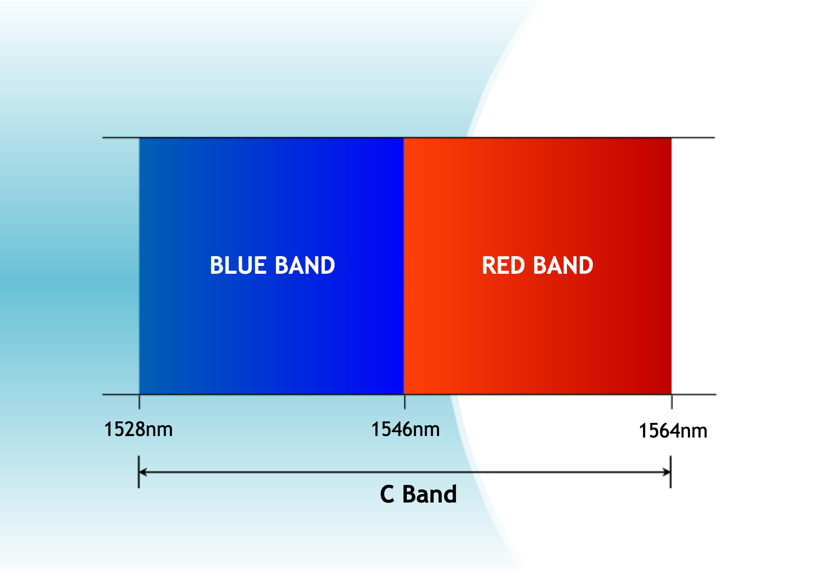
Figure 1: C-Band Red and Blue Band Division showing wavelength ranges and guard band
The ITU-standardized DWDM C-band spans from 1528.77 nm to 1563.86 nm, encompassing approximately 4.4 THz of optical bandwidth. This spectrum divides into two distinct regions: the red band, covering longer wavelengths from 1546.12 nm and above, and the blue band, comprising shorter wavelengths below 1546.12 nm. This division point is not arbitrary—it corresponds precisely to the optimal gain region of standard erbium-doped fiber amplifiers (EDFAs), the most widely deployed optical amplification technology in telecommunications networks.
Why Understanding Red and Blue Bands is Critical
For systems requiring limited channel counts (typically 8 to 40 wavelengths), deploying red band wavelengths enables the use of cost-optimized EDFAs with natural gain peaks aligned to longer wavelengths. This alignment reduces the complexity of gain flattening filters, minimizes amplified spontaneous emission (ASE) noise accumulation, and lowers overall capital expenditure. Conversely, blue band deployment becomes necessary when spectrum exhaustion in the red band drives capacity expansion or when specific transmission characteristics favor shorter wavelengths.
The terminology derives from astronomical Doppler shift principles, where "red-shift" describes electromagnetic radiation increasing in wavelength (shifting toward lower frequencies), and "blue-shift" represents wavelength decrease (shifting toward higher frequencies). In DWDM systems, this convention helps engineers quickly identify wavelength regions relative to a reference point—typically the center of the C-band or the EDFA gain peak.
This comprehensive guide explores the technical foundations, practical implications, and system design considerations for red and blue band wavelength allocation in modern DWDM networks. We examine EDFA gain profiles, ITU grid standards, nonlinear effects, filter design trade-offs, and real-world deployment strategies that leverage wavelength band characteristics for optimized network performance.
Historical Context and Evolution
Origins of Red-Shift and Blue-Shift Terminology
The concepts of red-shift and blue-shift originated in 19th-century physics, specifically from Austrian physicist Christian Doppler's 1842 observation of wave frequency changes in moving objects. Doppler demonstrated that sound waves from an approaching source compress, increasing frequency, while waves from a receding source stretch, decreasing frequency. This principle, extended to electromagnetic radiation, became foundational in astrophysics and spectroscopy.
In the visible spectrum, red occupies the longest wavelength region (approximately 620-750 nm), while blue resides at shorter wavelengths (approximately 450-495 nm). When astronomers observed distant galaxies, they noticed spectral lines shifting toward longer wavelengths—toward the "red end" of the spectrum—indicating those galaxies were moving away from Earth. This phenomenon, termed "cosmological redshift," became critical evidence for universal expansion. Conversely, objects moving toward an observer exhibit blue-shift, with spectral lines compressing toward shorter wavelengths.
Electromagnetic Spectrum Convention
The red-blue convention applies universally across the electromagnetic spectrum, not merely visible light. An infrared signal shifting to even longer wavelengths is "red-shifted" despite never appearing visibly red. Similarly, an ultraviolet signal shifting to shorter X-ray wavelengths is "blue-shifted" though it transcends human vision. This convention indicates directional movement in wavelength space: red means increasing wavelength (decreasing frequency), blue means decreasing wavelength (increasing frequency).
Adoption in Optical Networking
As DWDM technology emerged in the 1990s, optical engineers adopted the red-blue nomenclature to characterize wavelength regions within transmission bands. Early DWDM systems operated exclusively in the C-band (1530-1565 nm), where erbium-doped fiber amplifiers provided efficient amplification. Engineers observed that EDFAs exhibited wavelength-dependent gain profiles, with standard EDFA designs showing peak gain around 1532 nm under high pump inversion and around 1560 nm under moderate inversion.
The division point of 1546.12 nm emerged as a practical boundary because it approximately bisects the C-band and aligns with the transition in EDFA gain characteristics. Wavelengths above 1546.12 nm (red band) naturally align with the long-wavelength gain peak of EDFAs pumped at moderate inversion levels, requiring minimal gain flattening. Wavelengths below 1546.12 nm (blue band) require higher pump inversion or additional gain equalization to achieve flat amplification across all channels.
| Era | Technology Milestone | Red/Blue Band Impact |
|---|---|---|
| 1990-1995 | First commercial DWDM systems (8-16 channels) | Red band exclusively used due to EDFA gain alignment |
| 1996-2000 | 32-40 channel systems with gain-flattened EDFAs | Full C-band utilization, blue band deployment increases |
| 2001-2005 | 80-96 channel dense systems, L-band introduction | C-band red/blue distinction critical for amplifier design |
| 2006-2015 | 100G coherent transmission, flex-grid ROADMs | Spectral shaping enables efficient use of both bands |
| 2016-2025 | 400G/800G, constellation shaping, C+L systems | Red band remains cost-optimal for moderate channel counts |
Modern Relevance and Future Outlook
In contemporary optical networks, the red-blue distinction continues to influence system architecture despite advanced technologies that mitigate historical limitations. Modern EDFAs employ sophisticated gain-flattening filters, multi-stage designs, and dynamic gain control, enabling relatively uniform amplification across the entire C-band. However, fundamental physics—erbium ion energy levels, stimulated emission cross-sections, and spectral hole burning—still favor red band wavelengths for lowest noise figure and highest efficiency.
The future trajectory points toward flexible band utilization strategies. Software-defined optical networks with programmable amplifiers and adaptive modulation formats can dynamically allocate wavelengths to red or blue bands based on real-time conditions. Emerging technologies like multi-band EDFAs, Raman amplification, and parametric amplifiers may eventually neutralize band-specific advantages, but until these technologies achieve widespread cost-competitiveness, the red band's economic benefits remain compelling for many deployment scenarios.
Core Concepts and Fundamentals
ITU-T Grid and C-Band Structure
The International Telecommunication Union Telecommunication Standardization Sector (ITU-T) defines the DWDM frequency grid in Recommendation G.694.1. This standard establishes a fixed reference frequency of 193.1 THz (approximately 1552.52 nm) and specifies channel spacing in multiples of 12.5 GHz. Common spacings include 50 GHz (0.4 nm), 100 GHz (0.8 nm), and increasingly, flexible grid allocations in 12.5 GHz increments.
Figure 4: ITU-T DWDM frequency grid showing red and blue band channel allocation with 100 GHz spacing
The C-band extends from 1528.77 nm (196.1 THz) to 1563.86 nm (191.7 THz), providing approximately 4.4 THz of usable spectrum. Within this range, the red-blue division at 1546.12 nm (194.0 THz) creates two sub-bands with distinct characteristics:
C-Band Red Band (Long Wavelength)
Wavelength Range: 1546.12 nm to 1563.86 nm (191.7 to 194.0 THz)
Approximate Bandwidth: 2.3 THz
Channel Capacity (100 GHz spacing): ~23 channels
Channel Capacity (50 GHz spacing): ~46 channels
ITU Channel Numbers (100 GHz): Channels 20 to 43 (approximately)
Example Wavelengths: 1547.60 nm, 1549.40 nm, 1551.20 nm, 1553.00 nm, 1555.00 nm, 1557.00 nm, 1559.00 nm, 1561.53 nm
C-Band Blue Band (Short Wavelength)
Wavelength Range: 1528.77 nm to 1546.12 nm (194.0 to 196.1 THz)
Approximate Bandwidth: 2.1 THz
Channel Capacity (100 GHz spacing): ~21 channels
Channel Capacity (50 GHz spacing): ~42 channels
ITU Channel Numbers (100 GHz): Channels 44 to 64 (approximately)
Example Wavelengths: 1529.44 nm, 1531.24 nm, 1533.04 nm, 1535.04 nm, 1537.04 nm, 1539.04 nm, 1541.04 nm, 1543.84 nm
EDFA Gain Profile and Wavelength Dependence
Erbium-doped fiber amplifiers function through stimulated emission in erbium ions (Er³⁺) embedded in silica glass. When pumped with 980 nm or 1480 nm laser light, erbium ions transition to excited energy states. Signal photons at C-band wavelengths stimulate these excited ions to emit additional photons at the same wavelength, amplifying the signal.
The gain spectrum of an EDFA depends critically on the population inversion rate—the ratio of erbium ions in excited states versus ground states. The erbium ion's energy level structure consists of multiple Stark sublevels within both ground and excited states. At high population inversion (heavily pumped), the gain peak shifts toward shorter wavelengths (~1532 nm) as higher-energy sublevels become populated. At moderate inversion, the gain peak shifts toward longer wavelengths (~1560 nm) as lower-energy sublevels dominate.
Where:
G(λ) = wavelength-dependent gain
σe(λ) = emission cross-section at wavelength λ
σa(λ) = absorption cross-section at wavelength λ
N2 = population density of excited ions
N1 = population density of ground-state ions
L = length of erbium-doped fiber
For typical long-haul DWDM applications, EDFAs operate at moderate inversion to balance gain, noise figure, and efficiency. At this operating point, the natural gain profile exhibits a peak around 1555-1560 nm—squarely in the red band. Amplifying blue band wavelengths requires either:
Figure 2: EDFA gain profile showing natural preference for red band wavelengths at moderate population inversion
- Higher pump power to increase inversion and shift the gain peak shorter
- Longer erbium-doped fiber to accumulate sufficient gain at shorter wavelengths
- Gain-flattening filters to equalize the natural non-uniform gain profile
- Multi-stage designs with different inversion levels for different wavelength regions
Each approach increases system cost and complexity. For systems using only red band wavelengths, EDFAs can operate near their natural gain peak with minimal equalization, reducing both capital and operational expenses.
| EDFA Characteristic | Red Band (1546-1564 nm) | Blue Band (1529-1546 nm) |
|---|---|---|
| Natural Gain Alignment | Excellent (near gain peak) | Moderate (requires tuning) |
| Typical Gain (dB) | 28-32 dB | 24-28 dB |
| Noise Figure (dB) | 4.5-5.5 dB | 5.0-6.5 dB |
| Pump Efficiency | High (40-45%) | Moderate (35-40%) |
| Gain Flatness (unequalized) | 2-3 dB ripple | 3-5 dB ripple |
| Required EDF Length | 15-25 meters | 20-30 meters |
| Spectral Hole Burning | Lower impact | Higher impact |
Physical Basis: Wavelength and Frequency Relationships
The fundamental relationship between wavelength (λ) and frequency (f) of electromagnetic radiation is governed by the equation:
Where:
c = speed of light (≈ 3 × 10⁸ m/s in vacuum, ≈ 2 × 10⁸ m/s in optical fiber)
λ = wavelength (meters)
f = frequency (Hz)
This inverse relationship means longer wavelengths correspond to lower frequencies and vice versa. In DWDM systems:
- Red band wavelengths (longer λ, e.g., 1550-1564 nm) correspond to lower optical frequencies (192-194 THz)
- Blue band wavelengths (shorter λ, e.g., 1529-1546 nm) correspond to higher optical frequencies (194-196 THz)
The channel spacing in DWDM is typically specified in frequency units (GHz) rather than wavelength units (nm) because frequency spacing remains constant as channels propagate through fiber, while wavelength spacing can vary slightly due to chromatic dispersion and nonlinear effects.
Example:
λ = 1550 nm = 1550 × 10⁻⁹ m
f = (3 × 10⁸) / (1550 × 10⁻⁹) = 193.548 THz
L-Band Red and Blue Division
Figure 6: Complete optical fiber transmission spectrum showing all wavelength bands with C-Band red/blue division and fiber loss profile
The concept of red and blue bands extends beyond the C-band to other transmission windows. The L-band (long band), spanning 1565-1625 nm (191.7-187.5 THz), represents the next logical capacity expansion when C-band spectrum is exhausted. The L-band also exhibits red and blue sub-band characteristics:
L-Band Red Band
Wavelength Range: 1589 nm to 1603 nm
Characteristics: Aligns with L-band EDFA gain peak, lowest attenuation in L-band
L-Band Blue Band
Wavelength Range: 1570 nm to 1584 nm
Characteristics: Closer to C-band, higher EDFA efficiency than deep L-band
L-band EDFAs face greater challenges than C-band amplifiers. The erbium ion exhibits lower emission cross-sections in the L-band, requiring longer erbium-doped fiber lengths (50-100 meters vs. 15-30 meters for C-band) and higher pump powers. Additionally, L-band amplifiers demonstrate increased temperature sensitivity and greater spectral hole burning effects. Despite these challenges, L-band deployment becomes economically justified when C-band capacity constraints prevent meeting traffic demands without installing additional fiber pairs.
Technical Architecture and Components
DWDM System Architecture with Band-Specific Components
A complete DWDM transmission system comprises several key subsystems, each influenced by the red-blue band distinction. The fundamental architecture includes transponders (converting client signals to DWDM wavelengths), multiplexers (combining multiple wavelengths), optical amplifiers (compensating for fiber loss), transmission fiber, demultiplexers (separating wavelengths), and receivers.
Figure 3: Complete DWDM system architecture showing red and blue band wavelength paths through multiplexing, amplification, and transmission
Transponder Considerations
Transponders generate the DWDM wavelengths using tunable or fixed-wavelength lasers. For red band operation, distributed feedback (DFB) lasers operating at 1550-1564 nm offer excellent performance characteristics with mature manufacturing processes. Blue band wavelengths (1529-1546 nm) require careful laser design to maintain frequency stability, as shorter wavelengths exhibit greater thermal drift effects.
Temperature Coefficient: ~0.1 nm/°C for typical DFB lasers. Red band lasers at 1555 nm experiencing a 10°C temperature swing drift approximately 1 nm (125 GHz), potentially crossing into adjacent channels. Blue band lasers at 1535 nm under identical conditions drift similarly in wavelength but represent a larger frequency shift (~130 GHz), requiring tighter temperature control.
Multiplexer and Demultiplexer Filter Design
Optical multiplexers and demultiplexers separate or combine wavelengths using wavelength-selective filters. The most common technologies include thin-film filters (TFF), arrayed waveguide gratings (AWG), and fiber Bragg gratings (FBG). Filter design requirements differ between red and blue band operation:
| Filter Characteristic | Red Band Filters | Blue Band Filters |
|---|---|---|
| Center Wavelength Stability | 0.05 nm/°C typical | 0.04 nm/°C (tighter control needed) |
| Passband Width (100 GHz channels) | ±0.25 nm (31 GHz) | ±0.22 nm (33 GHz at shorter λ) |
| Insertion Loss | 3.0-4.5 dB | 3.5-5.0 dB |
| Crosstalk Isolation | >30 dB adjacent channel | >32 dB (higher density at shorter λ) |
| Manufacturing Tolerance | Standard (±0.1 nm) | Tighter (±0.08 nm) |
The blue band's shorter wavelengths necessitate tighter manufacturing tolerances because a fixed wavelength deviation (e.g., 0.1 nm) represents a larger fraction of the channel spacing at higher frequencies. Additionally, blue band filters may experience greater temperature sensitivity requiring active thermal control or athermal designs.
Amplifier Architecture for Band-Specific Operation
Modern DWDM amplifiers employ several architectural approaches to accommodate red and blue band wavelengths effectively:
Single-Stage Red Band Optimized EDFA
Configuration: 15-20m erbium-doped fiber, 980nm pump (150-250mW), minimal gain flattening
Performance: 25-30 dB gain, 4.5-5.5 dB noise figure, excellent efficiency
Application: Cost-sensitive metro and regional networks with limited channel counts (8-32 wavelengths) exclusively in red band
Dual-Stage Full C-Band EDFA
Configuration: Two erbium-doped fiber stages with mid-stage VOA (variable optical attenuator) and gain-flattening filter
Performance: 20-28 dB gain with ±0.5 dB flatness across entire C-band, 5.0-6.0 dB noise figure
Application: Long-haul and submarine systems requiring full C-band utilization (red and blue bands)
Hybrid Raman + EDFA
Configuration: Distributed Raman amplification in transmission fiber followed by discrete EDFA
Performance: Improved OSNR through distributed gain, 3-5 dB lower noise figure effective
Application: Ultra-long-haul systems where blue band channels would otherwise suffer excessive OSNR penalty
Gain Flattening Filter Requirements
Gain flattening filters (GFFs) compensate for the wavelength-dependent gain variation of EDFAs. These filters exhibit an inverse spectral response to the EDFA's natural gain profile, attenuating wavelengths with higher natural gain to equalize all channels. Red band operation significantly reduces GFF complexity and insertion loss:
| Parameter | Red Band Only | Full C-Band |
|---|---|---|
| GFF Attenuation Range | 2-3 dB | 4-6 dB |
| GFF Insertion Loss | 1.5-2.0 dB | 2.5-3.5 dB |
| Filter Complexity | Single Bragg grating | Multi-cavity thin-film or cascaded gratings |
| Temperature Sensitivity | Low (passive compensation) | Moderate (active or athermal design) |
| Cost Impact | $200-500 per amplifier | $800-1500 per amplifier |
For systems deploying only red band wavelengths, the natural EDFA gain profile exhibits relatively flat response (2-3 dB variation) across the band, enabling simple, low-loss flattening filters. Full C-band systems require sophisticated filters to compensate for 5-8 dB gain variation between blue and red extremes, increasing both cost and insertion loss.
Fiber Nonlinear Effects and Wavelength Dependence
Optical fiber exhibits wavelength-dependent nonlinear effects that influence red and blue band performance. The most significant nonlinearities in DWDM systems include four-wave mixing (FWM), cross-phase modulation (XPM), self-phase modulation (SPM), and stimulated Raman scattering (SRS).
Stimulated Raman Scattering: SRS transfers power from shorter wavelengths (blue band) to longer wavelengths (red band) through inelastic scattering. In C+L band systems, this effect creates a systematic power tilt favoring red band channels. The Raman gain coefficient peaks approximately 13 THz (100 nm) below the pump wavelength, meaning blue band C-band channels (~1530 nm) efficiently pump red band C-band channels (~1560 nm).
SRS-induced power transfer accumulates with fiber length and increases with total optical power. In a fully loaded C-band system with 50 channels at 0 dBm per channel, SRS can create 4-6 dB of power tilt across an 80 km span, with blue channels depleted and red channels amplified. This effect necessitates pre-emphasis (launching blue channels at higher power) or dynamic gain control to maintain channel uniformity.
Four-Wave Mixing: FWM generates spurious mixing products at frequencies fijk = fi + fj - fk when multiple wavelengths propagate simultaneously. FWM efficiency depends on phase-matching conditions, which are influenced by chromatic dispersion. Interestingly, FWM products from blue band channels tend to fall on-grid more frequently than products from red band channels due to dispersion characteristics of standard single-mode fiber (SMF).
In SMF, chromatic dispersion increases approximately linearly from 15 ps/(nm·km) at 1530 nm to 18 ps/(nm·km) at 1565 nm. This positive dispersion slope provides slightly better FWM suppression in the red band compared to the blue band, particularly for closely spaced channels (50 GHz spacing).
Mathematical Models and Formulas
OSNR Calculation for Red vs Blue Bands
Optical Signal-to-Noise Ratio (OSNR) represents the fundamental figure of merit for optical transmission quality. OSNR degrades as signals traverse multiple amplifiers, with each amplifier adding amplified spontaneous emission (ASE) noise. The accumulated OSNR after N amplifier stages is given by:
In dB notation:
OSNRdB = Psignal,dBm - 10·log10(N) - PASE,dBm
The ASE power spectral density generated by a single EDFA is:
Where:
nsp = spontaneous emission factor (population inversion parameter)
h = Planck's constant (6.626 × 10⁻³⁴ J·s)
ν = optical frequency (Hz)
G = amplifier gain (linear)
Δνref = reference bandwidth (typically 12.5 GHz or 0.1 nm)
The spontaneous emission factor nsp depends on population inversion and differs between wavelengths. For red band wavelengths operating near the EDFA's natural gain peak, nsp ≈ 1.3-1.5 (corresponding to 3-4 dB noise figure). For blue band wavelengths, nsp ≈ 1.6-2.0 (corresponding to 4-6 dB noise figure).
Practical Example: Consider a 10-span system with 80 km spans, requiring 10 optical line amplifiers (OLAs):
Figure 5: OSNR degradation comparison showing red band's consistent 1.0 dB advantage over blue band across multiple amplifier spans
- Red Band (1555 nm): Amplifier NF = 4.5 dB, Gain = 18 dB (to compensate span loss)
- Blue Band (1535 nm): Amplifier NF = 5.5 dB, Gain = 18 dB
With launched power of +2 dBm per channel:
OSNRred = 2 + 58 - 4.5 - 10 = 45.5 dB
OSNRblue = 2 + 58 - 5.5 - 10 = 44.5 dB
The red band channel achieves 1.0 dB better OSNR than the blue band channel due to superior EDFA noise figure.
Chromatic Dispersion Calculation
Chromatic dispersion causes pulse broadening as different wavelength components travel at different velocities in optical fiber. Standard single-mode fiber (SMF-28) exhibits dispersion parameter D(λ) that varies with wavelength:
For SMF-28:
λ0 = 1310 nm (zero-dispersion wavelength)
D0 ≈ 0 ps/(nm·km) at λ0
S0 ≈ 0.092 ps/(nm²·km) (dispersion slope)
At C-band wavelengths:
- Blue Band (1535 nm): D = 0 + 0.092 × (1535 - 1310) = 15.7 ps/(nm·km)
- Red Band (1555 nm): D = 0 + 0.092 × (1555 - 1310) = 17.5 ps/(nm·km)
Accumulated dispersion after distance L:
Example for 800 km:
Blue Band: Dtotal = 15.7 × 800 = 12,560 ps/nm
Red Band: Dtotal = 17.5 × 800 = 14,000 ps/nm
The blue band accumulates approximately 10% less chromatic dispersion than the red band over equivalent distances. For 10 Gbps NRZ modulation, the dispersion penalty becomes significant beyond ~50,000 ps/nm (uncompensated), meaning blue band channels can tolerate slightly longer reaches before requiring dispersion compensation. However, modern coherent systems with digital signal processing (DSP) compensate chromatic dispersion electronically, largely neutralizing this advantage.
Stimulated Raman Scattering Power Transfer
SRS transfers power from shorter wavelength (pump) channels to longer wavelength (Stokes) channels. The power transfer between two wavelengths separated by frequency shift Δν is governed by:
Where:
gR = Raman gain coefficient ≈ 1 × 10⁻¹³ m/W at peak (13 THz shift)
Leff = effective fiber length ≈ L × [1 - exp(-αL)] / α
PStokes = power of longer wavelength channel
In a full C-band DWDM system with channels spanning 1530-1565 nm (35 nm or ~4.4 THz), the frequency separation between extreme blue and red channels approaches the Raman gain peak (~13 THz for 100 nm separation in wavelength). While not at peak efficiency, SRS still causes measurable power transfer.
Practical Impact: In an 80 km span with 40 channels at +1 dBm per channel, SRS creates approximately 1-2 dB of power tilt across the C-band, with blue band channels losing power and red band channels gaining power. This effect accumulates over multiple spans, requiring amplifier pre-emphasis or dynamic equalization to maintain channel uniformity.
Types, Variations, and Classifications
DWDM System Classifications by Band Usage
| System Type | Band Utilization | Typical Application | Advantages | Limitations |
|---|---|---|---|---|
| Red Band Only | 1546-1564 nm ~20-25 channels (100 GHz) |
Metro, regional networks Cost-sensitive deployments |
Lowest cost per channel Simple EDFAs Minimal GFF complexity |
Limited capacity Spectrum inefficient |
| Full C-Band | 1529-1564 nm ~40-50 channels (100 GHz) |
Long-haul networks High-capacity metro |
Double capacity vs red-only Standard technology Wide vendor support |
Higher amplifier cost Complex GFF required SRS tilt management |
| C+L Dual Band | 1529-1625 nm ~80-100 channels (100 GHz) |
Submarine cables Ultra-high-capacity backbone |
Maximum capacity Fiber efficiency |
Highest cost Complex amplification Severe SRS tilt L-band lower efficiency |
| Flex-Grid Variable | Dynamic allocation 12.5 GHz granularity |
Software-defined networks Elastic optical networks |
Spectrum efficiency Adaptive capacity Mixed data rates |
Complex control plane Expensive ROADMs Fragmentation challenges |
EDFA Architectures for Different Band Requirements
Type 1: Single-Stage Red Band EDFA
Configuration: Single erbium-doped fiber section with 980 nm pump
Wavelength Coverage: 1546-1564 nm (red band optimized)
Typical Specifications:
- Gain: 25-30 dB
- Noise Figure: 4.5-5.5 dB
- Gain Flatness: ±1.5 dB (unequalized), ±0.5 dB (with simple GFF)
- EDF Length: 15-20 meters
- Pump Power: 150-250 mW
Cost Impact: Baseline (1.0x)
Type 2: Dual-Stage Full C-Band EDFA
Configuration: Two EDF stages with mid-stage access for VOA and GFF
Wavelength Coverage: 1529-1564 nm (full C-band)
Typical Specifications:
- Gain: 20-28 dB (power-dependent)
- Noise Figure: 5.0-6.5 dB
- Gain Flatness: ±0.5 dB (with sophisticated GFF)
- Total EDF Length: 25-35 meters
- Pump Power: 300-500 mW (dual pumps)
Cost Impact: 1.6-2.0x vs Type 1
Type 3: C+L Dual-Band Amplifier System
Configuration: Separate C-band and L-band EDFA modules with band splitter/combiner
Wavelength Coverage: 1529-1625 nm (C+L bands)
Typical Specifications:
- C-band Module: Similar to Type 2
- L-band Module: 18-25 dB gain, 5.5-7.0 dB NF
- Total System Gain: 18-25 dB (balanced)
- L-band EDF Length: 50-100 meters
- Total Pump Power: 600-1000 mW
Cost Impact: 3.5-5.0x vs Type 1
The cost progression from red-band-only to full C-band to C+L systems is non-linear, with C+L systems disproportionately expensive due to L-band EDFA challenges (longer fiber, higher pump power, lower efficiency, greater temperature sensitivity).
Interactive Simulators
Practical Applications and Case Studies
Case Study 1: Regional Network Red Band Optimization
Challenge
A major telecommunications provider needed to expand capacity on a regional optical network connecting 12 cities across 800 km. The existing infrastructure supported 16 wavelengths (10G channels) operating in the red band (1550-1562 nm). Traffic growth projections indicated requirement for 24-32 wavelengths within 18 months.
Options Evaluated
- Option A: Expand to full C-band (40 channels capability), requiring all EDFA upgrades
- Option B: Add more red band channels with existing EDFAs, limited to 25 total channels
- Option C: Install parallel fiber pair with separate red band system
Solution
The provider selected Option B (maximized red band utilization) with the following implementation:
- Reduced channel spacing from 100 GHz to 50 GHz in red band
- Added minor gain-flattening filter enhancements to existing EDFAs
- Upgraded transponders to support 50 GHz spacing
- Total capacity increased to 40 wavelengths (red band: 25 channels, keeping blue band reserved for future)
Results
Cost Impact: $2.3M for Option B vs. $6.8M for Option A (66% savings)
Timeline: 4 months deployment vs. 12 months for full EDFA replacement
Performance: Average OSNR 32.5 dB (exceeds 10G requirements of 18 dB by 14.5 dB margin)
Future-proofing: Blue band remains available for next capacity expansion without major infrastructure changes
Case Study 2: Submarine Cable C+L Band Deployment
Challenge
A consortium building a 6,000 km transoceanic submarine cable system needed to maximize capacity within severe cost, power, and physical space constraints. The system required support for 100 wavelengths at 100G per channel (10 Tbps total capacity) with 15-year service life.
Technical Approach
Full C+L band deployment with advanced amplification:
- C-band: 50 channels in full C-band (1530-1565 nm) using dual-stage EDFAs
- L-band: 50 channels in L-band (1570-1610 nm) with dedicated L-band EDFAs
- Amplifier spacing: 50 km (vs. 80 km typical for terrestrial)
- Raman assistance: Backward-pumped Raman amplification in both bands
- SRS management: Pre-emphasis launching C-band blue channels at +2 dBm, red channels at 0 dBm
Band-Specific Challenges
C-Band Red vs Blue: Minimal difference due to sophisticated amplification; both bands achieved 24 dB OSNR
L-Band Challenges: Required 50% longer EDF (70m vs. 45m for C-band), 40% higher pump power (800mW vs. 570mW), resulted in 1.2 dB higher noise figure (6.8 dB vs. 5.6 dB in C-band)
Results
Capacity: 10 Tbps achieved (100 × 100G channels)
OSNR Performance: C-band: 23-25 dB; L-band: 21-23 dB (both adequate for 100G PM-QPSK modulation requiring 12-14 dB OSNR)
Cost: Approximately $350M total system cost, with C+L amplification representing ~$85M (24%)
Alternative Analysis: C-band-only deployment would have required 200 channels at 50 GHz spacing or wavelength-selective switches—economically infeasible at time of deployment
Case Study 3: Data Center Interconnect Migration Strategy
Challenge
A hyperscale cloud provider operates multiple DCI links connecting data centers across metropolitan areas (40-120 km distances). Initial deployment used 8 wavelengths (100G) in red band. Explosive growth required 10x capacity increase to support AI/ML workloads, object storage replication, and live migration traffic.
Migration Strategy
Phase 1 (Year 1): Maximize red band capacity
- Deployed 50 GHz channel spacing with coherent 200G channels
- Achieved 20 wavelengths × 200G = 4 Tbps per fiber pair
- Used existing red band optimized EDFAs with minor tuning
Phase 2 (Year 2): Add blue band capacity
- Upgraded EDFAs to full C-band capability
- Added 20 blue band channels at 50 GHz spacing
- Total capacity: 40 wavelengths × 200G = 8 Tbps per fiber pair
Phase 3 (Year 3): Advanced modulation and flex-grid
- Migrated to 400G coherent with flex-grid allocation (75 GHz per channel)
- Achieved 50 channels × 400G = 20 Tbps per fiber pair
- Spans <120 km enabled aggressive spectral efficiency
Key Insights
Red Band Advantage: Phase 1 implementation with red-only channels provided 75% of required capacity at 30% lower cost than immediate full C-band deployment
Graceful Upgrade Path: Phased approach enabled capacity expansion aligned with actual demand growth, avoiding over-provisioning
Metro Distance Benefit: Short distances (40-120 km) with high OSNR (>30 dB) enabled advanced modulation formats, where band-specific OSNR differences became negligible
Troubleshooting Guide: Common Band-Specific Issues
| Symptom | Probable Cause | Diagnostic Steps | Resolution |
|---|---|---|---|
| Blue band channels exhibit 2-4 dB higher BER than red band | Inadequate EDFA gain for blue wavelengths | Measure OSNR across all channels; verify EDFA pump power and gain profile | Increase pump power to raise inversion; add/tune gain-flattening filter; consider two-stage EDFA upgrade |
| Progressive power tilt developing over time (blue channels losing power) | Stimulated Raman Scattering transferring power from blue to red | Monitor channel powers at multiple points; calculate total launched power | Implement pre-emphasis (launch blue channels at higher power); enable dynamic channel power management; consider Raman amplification |
| Intermittent errors on blue band channels only | Temperature-dependent filter drift affecting shorter wavelengths | Check mux/demux temperatures; monitor errors vs. temperature | Install athermal filters or active temperature control; verify filter specifications match channel grid |
| Red band channels near 1562 nm show elevated FWM products | Reduced dispersion at longer wavelengths improving FWM phase matching | Spectrum analyzer to identify FWM products; calculate FWM efficiency | Increase channel spacing to 100 GHz; reduce channel power; consider dispersion-shifted fiber for affected spans |
| Cannot achieve flat gain across full C-band despite GFF | Spectral hole burning from unequal channel powers | Measure individual channel powers; identify high-power channels causing gain depression | Balance channel powers before amplifier; use mid-stage VOA with dynamic control; consider multiple lower-gain stages |
Best Practices and Design Recommendations
When to Choose Red Band Only
Recommended for:
- New deployments requiring ≤25 channels (100 GHz spacing) or ≤50 channels (50 GHz spacing)
- Cost-sensitive projects where capital expenditure minimization is prioritized
- Networks with moderate expected growth (2-3x over 5-7 years)
- Metro and regional networks where fiber scarcity is not a constraint
- Systems using older 10G or 40G transponder technology with relaxed OSNR requirements
Advantages: 20-40% lower cost per amplifier, simpler operations, better OSNR margins, lower power consumption
Limitations: Limited capacity expansion path, inefficient spectrum utilization if multiple fibers available
When to Deploy Full C-Band
Recommended for:
- High-capacity backbone networks requiring 40-96 channels
- Environments where fiber installation costs exceed equipment costs significantly
- Long-haul systems (>1000 km) where maximizing single-fiber capacity justifies higher amplifier costs
- Future-proof deployments anticipating 5-10x capacity growth
- Networks planning eventual L-band expansion (C-band serves as foundation)
Advantages: Maximum C-band capacity, proven technology, vendor interoperability, straightforward L-band upgrade path
Considerations: Higher initial cost, increased operational complexity, requires sophisticated monitoring
Hybrid Strategy: Start Red, Expand to Full C-Band
Optimal approach for many scenarios:
- Phase 1: Deploy red band channels with future-ready amplifier shelves
- Phase 2: Add blue band capability when red band capacity approaches 70-80% utilization
- Benefits: Defers C-band investment until needed, aligns capital expenditure with revenue growth, maintains migration path
- Requirements: Plan for full C-band amplifiers from start (avoid needing replacements), install filters with adequate bandwidth, allocate rack space for future modules
Summary: Key Takeaways
Red-Blue Convention
The red-blue nomenclature originates from electromagnetic spectrum physics, with "red" indicating longer wavelengths (lower frequencies) and "blue" indicating shorter wavelengths (higher frequencies). This convention applies universally across the spectrum, not just visible light.
ITU C-Band Division
The C-band divides at approximately 1546.12 nm: red band covers 1546-1564 nm (~23-25 channels at 100 GHz spacing), while blue band spans 1529-1546 nm (~21-23 channels). This division aligns with EDFA gain characteristics.
EDFA Efficiency
Erbium-doped fiber amplifiers naturally favor red band wavelengths, exhibiting 0.5-1.5 dB better noise figure and requiring less complex gain flattening. This translates to superior OSNR performance and lower system cost for red-only deployments.
Cost-Capacity Trade-off
Red band systems cost 20-40% less per amplifier than full C-band systems. For networks requiring ≤25 channels, red band optimization provides the most economical solution without compromising performance.
Nonlinear Effects
Stimulated Raman scattering systematically transfers power from blue to red bands in multi-wavelength systems, creating power tilt that requires management through pre-emphasis or dynamic equalization in full C-band deployments.
Filter Considerations
Blue band filters require tighter manufacturing tolerances and more precise temperature control than red band filters due to wavelength-frequency relationships and higher channel density at shorter wavelengths.
Dispersion Characteristics
Blue band wavelengths experience ~10% less chromatic dispersion than red band in standard single-mode fiber, though this advantage is largely neutralized by modern coherent receivers with electronic dispersion compensation.
Deployment Strategy
Optimal strategy for many networks: start with red band channels for cost efficiency, maintain upgrade path to full C-band as capacity demands grow. This approach aligns capital expenditure with revenue growth.
L-Band Extension
L-band (1565-1625 nm) also divides into red (1589-1603 nm) and blue (1570-1584 nm) sub-bands, with similar EDFA efficiency differences. L-band deployment is economically justified only when C-band capacity is exhausted.
Future Outlook
While advanced technologies like multi-band amplifiers and coherent DSP are reducing band-specific differences, fundamental physics ensures red band's efficiency advantages will persist, particularly for cost-sensitive deployments requiring moderate channel counts.
For educational purposes in optical networking and DWDM systems
Note: This guide is based on industry standards, best practices, and real-world implementation experiences. Specific implementations may vary based on equipment vendors, network topology, and regulatory requirements. Always consult with qualified network engineers and follow vendor documentation for actual deployments.

Optical Communications & Network Automation Expert | Author of 3 Books for Optical Engineers | Founder, MapYourTech
Optical networking engineer with nearly two decades of experience across DWDM, OTN, coherent optics, submarine systems, and cloud infrastructure. Founder of MapYourTech. Read full bio →
Follow on LinkedIn