27 min read

Digital Diagnostics Monitoring (DDM): Real-Time Transceiver Health Monitoring
Introduction
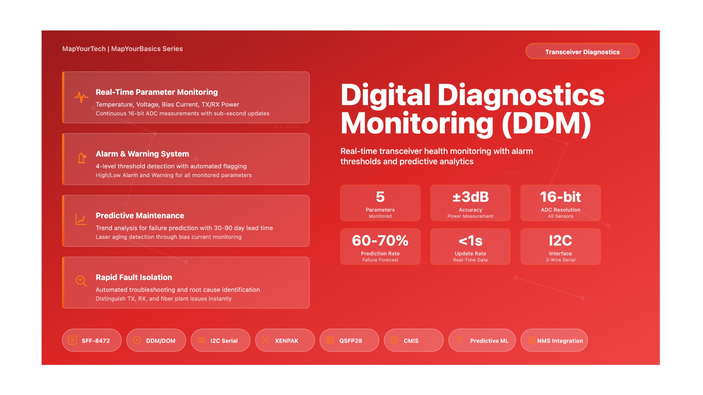
Digital Diagnostics Monitoring (DDM), also known as Digital Optical Monitoring (DOM), represents a critical advancement in optical networking technology. This capability provides real-time access to vital operating parameters within optical transceivers, allowing network operators and engineers to monitor the health and performance of their optical links before problems become service-affecting failures.
Modern optical networks rely on thousands of optical transceivers operating continuously under varying environmental conditions. Without DDM, network operators would be flying blind, only discovering transceiver issues after complete failure or severe performance degradation. DDM changes this by providing continuous visibility into key performance indicators including temperature, supply voltage, laser bias current, transmitted optical power, and received optical power. This proactive monitoring approach has become essential for maintaining high-availability networks and reducing mean time to repair (MTTR) when issues do occur.
The technology operates through a sophisticated system of internal sensors, analog-to-digital converters, and a standardized digital interface. The transceiver continuously measures critical parameters and makes this data available to the host system through a serial interface. Beyond simple measurement, DDM implements a comprehensive alarm and warning system with factory-programmed thresholds that alert operators when parameters drift outside normal operating ranges.
This article provides a comprehensive exploration of DDM technology, covering its fundamental principles, technical architecture, monitored parameters, alarm systems, practical applications, and troubleshooting techniques. Whether you're a network engineer implementing DDM monitoring for the first time, a NOC operator interpreting alarm data, or a network architect designing monitoring systems, this guide will provide the technical knowledge needed to effectively use DDM capabilities.
Why DDM is Essential
DDM provides several critical benefits for optical network operations:
- Predictive Maintenance: Identify transceivers trending toward failure before they impact service
- Rapid Troubleshooting: Quickly isolate the root cause of link issues (transmitter, receiver, fiber, or external)
- Performance Optimization: Fine-tune optical power levels across the network for optimal performance
- Inventory Management: Verify transceiver specifications and track operational history
- Environmental Monitoring: Detect equipment room temperature issues before they cause widespread failures
1. Historical Evolution and Standards Development
1.1 Early Optical Transceivers
The first generation of optical transceivers, including GBIC (Gigabit Interface Converter) modules introduced in the late 1990s, had no diagnostic capabilities. When a link failed, troubleshooting required swapping transceivers, testing fiber, and often bringing expensive optical test equipment to the site. This reactive approach resulted in extended downtime and inefficient use of engineering resources.
GBIC modules provided basic identification data through a serial EEPROM, allowing the host system to read vendor name, part number, and wavelength information. However, there was no ability to monitor real-time operating conditions. Engineers could not determine if a transceiver was running hot, if laser power was degrading, or if received signal levels were marginal.
1.2 Introduction of SFF-8472 Standard
The breakthrough came with the development of the SFF-8472 specification, "Digital Diagnostic Monitoring Interface for Optical Transceivers." This Multi-Source Agreement (MSA) defined a standardized method for transceivers to report real-time operating parameters. The standard was initially developed for SFP (Small Form-factor Pluggable) transceivers but its principles were later extended to other form factors.
SFF-8472 introduced several key innovations:
- A standardized 256-byte memory map accessible via I2C interface
- Definition of monitored parameters and their data formats
- Alarm and warning thresholds for each monitored parameter
- Calibration methods to ensure measurement accuracy
- Backward compatibility with existing serial ID specifications
The standard defined two I2C addresses: A0h for basic identification data (maintaining compatibility with earlier specifications) and A2h for diagnostic monitoring data. This two-address scheme allowed older host systems without DDM support to continue functioning while enabling newer systems to take advantage of diagnostic capabilities.
1.3 Extension to Other Form Factors
Following the success of SFF-8472 for SFP modules, similar diagnostic capabilities were incorporated into standards for other transceiver form factors. The XENPAK MSA included DDM specifications accessed through MDIO/MDC interface instead of I2C. XFP transceivers adopted INF-8077i, which provided even more comprehensive monitoring including per-lane diagnostics for multi-lane implementations.
Modern high-speed transceivers including QSFP28, QSFP-DD, and OSFP modules have further enhanced DDM capabilities. These newer standards provide lane-specific monitoring for parallel optics, more detailed alarm information, and faster update rates for monitoring data. The principles established in SFF-8472, however, remain fundamental across all implementations.
2. Fundamental Principles of DDM Operation
2.1 Physical Measurement Mechanisms
DDM operates by measuring analog signals within the transceiver using dedicated monitoring circuits and sensors. These analog signals are then converted to digital values through an analog-to-digital converter (ADC), typically with 16-bit resolution. The digitized values are processed through calibration algorithms and stored in accessible memory locations.
Each monitored parameter uses a specific measurement technique:
Temperature Measurement
Temperature monitoring uses an integrated temperature sensor, typically a semiconductor junction or thermistor located near the laser and critical electronic components. The sensor generates a voltage proportional to temperature, which is measured by the ADC. Temperature readings are critical because laser performance, lifetime, and threshold current are all temperature-dependent.
Supply Voltage Monitoring
The transceiver monitors its supply voltage (typically 3.3V or 3.135V-3.465V range) using a simple voltage divider network connected to the ADC input. This measurement detects power supply problems, inadequate filtering, or voltage sag under load conditions.
Laser Bias Current
Laser bias current is measured by monitoring the voltage drop across a small series resistor in the laser drive circuit. The bias current indicates the electrical drive level required to maintain constant optical output power. As lasers age or temperature changes, the automatic power control (APC) circuit must adjust bias current to maintain output power, making this parameter an excellent indicator of laser health.
Transmit Optical Power
TX power is measured using a photodiode tap that samples a small portion (typically 1-5%) of the laser output before it enters the fiber. This monitor photodiode generates a current proportional to optical power, which is converted to voltage and measured. The digital value is then calibrated to represent absolute optical power in milliwatts or dBm.
Receive Optical Power
RX power measurement samples the current from the main receiver photodiode, typically through a current mirror or sense resistor. Since the photodiode current is directly proportional to incident optical power, this provides an accurate measurement of received signal strength. This is one of the most useful DDM parameters for troubleshooting fiber plant issues.
2.2 ADC and Digital Processing
The heart of the DDM system is the Digital Diagnostics Transceiver Controller (DDTC), which typically includes a 16-bit ADC capable of measuring multiple analog inputs sequentially. The 16-bit resolution provides adequate dynamic range to cover the full operating range of each parameter while maintaining reasonable accuracy.
The ADC conversion process follows this sequence:
- An analog multiplexer sequentially selects each monitored parameter
- The selected signal is held steady during the conversion period
- The ADC performs the conversion (typically taking 10-100 microseconds)
- The digital result is passed to the calibration engine
- The calibrated value is stored in the appropriate memory location
Update rates for monitored parameters are typically in the range of 100ms to 1 second, fast enough for real-time monitoring but slow enough to filter out noise and transients. Some advanced implementations provide faster update rates for critical parameters like receive power.
2.3 Calibration Methods
Two calibration methods are defined in the DDM specifications: internal calibration and external calibration.
Internal Calibration
Internal calibration is the most common method in modern transceivers. The DDTC includes calibration coefficients programmed during manufacturing that convert raw ADC readings to calibrated values. For temperature, a simple linear equation is typically used:
T = Tslope × ADCraw + Toffset

Where:
  T = Calibrated temperature (°C)
  Tslope = Temperature calibration slope
  ADCraw = Raw ADC reading
  Toffset = Temperature calibration offset
For optical power measurements, the calibration is more complex to account for non-linearities in photodiode response:
PRX = Rx_PWR4 × ADC4 + Rx_PWR3 × ADC3 + Rx_PWR2 × ADC2 + Rx_PWR1 × ADC + Rx_PWR0

Where:
  PRX = Received optical power (mW)
  Rx_PWRn = Calibration coefficients (n = 0 to 4)
  ADC = Raw ADC reading

Note: Polynomial fit accounts for photodiode non-linearity
External Calibration
External calibration is a simpler approach where the transceiver manufacturer characterizes the module during production and stores pre-calculated values in the EEPROM. The host system reads these values directly without performing calculations. While easier to implement in the transceiver, this method typically requires more memory storage and may be less accurate over the full temperature range.
3. Monitored Parameters and Data Formats
3.1 Parameter Overview
DDM systems monitor five primary parameters, each serving a specific diagnostic purpose. The following table summarizes these parameters, their typical ranges, and measurement accuracy requirements:
| Parameter | Typical Range | Accuracy | Units | Primary Use |
|---|---|---|---|---|
| Temperature | 0°C to 70°C (commercial) -5°C to 85°C (extended) -40°C to 85°C (industrial) |
±3°C to ±5°C | °C | Environmental monitoring, thermal management |
| Supply Voltage | 3.135V to 3.465V | ±0.1V | V | Power supply health, voltage sag detection |
| Laser Bias Current | 5mA to 100mA (typical) Varies by laser type |
±10% | mA | Laser aging, temperature effects, end-of-life prediction |
| TX Optical Power | -10dBm to +5dBm Varies by standard |
±2dB to ±3dB | dBm or mW | Transmitter health, fiber connection quality |
| RX Optical Power | -40dBm to +5dBm Wide dynamic range |
±2dB to ±3dB | dBm or mW | Link budget analysis, fiber plant troubleshooting |
3.2 Temperature Monitoring
Temperature is reported as a 16-bit signed two's complement integer. The most significant byte (MSB) represents the integer portion of the temperature in degrees Celsius, while the least significant byte (LSB) provides fractional resolution. Each LSB increment represents 1/256°C, providing theoretical resolution of approximately 0.004°C, though actual accuracy is typically ±3°C to ±5°C.
Temperature monitoring serves multiple purposes. First, it allows operators to detect equipment room cooling failures before temperatures reach levels that trigger shutdown or cause permanent damage. Second, temperature trends can identify modules operating outside their specified range, which may experience reduced reliability or accelerated aging. Third, temperature correlates with other parameters, particularly laser bias current, and understanding this relationship aids troubleshooting.
Temperature Range Classifications
Commercial: 0°C to 70°C - Standard office and controlled environment deployments
Extended: -5°C to 85°C - Outdoor cabinets with some environmental control
Industrial: -40°C to 85°C - Harsh environments, extreme climates, minimal climate control
3.3 Supply Voltage Monitoring
Supply voltage is represented as a 16-bit unsigned integer where the full 16-bit value (0-65535) maps to 0V to 6.55V with 0.1mV resolution (LSB = 0.1mV). Normal operating voltage for most transceivers is 3.3V ±0.165V (3.135V to 3.465V).
Voltage monitoring detects several potential issues. A slowly decreasing voltage over time might indicate power supply aging or inadequate capacity. Voltage that varies with data activity suggests insufficient filtering or current capacity in the supply distribution. Voltage outside the specified range can cause erratic behavior, increased bit error rate, or complete transceiver failure.
3.4 Laser Bias Current
Laser bias current is reported as a 16-bit unsigned integer. Different transceiver types use different scaling factors, typically either 2µA or 10µA per LSB. The specific scaling factor used is indicated in the transceiver's capability registers.
Laser bias current is one of the most valuable parameters for predicting transceiver end-of-life. As a laser ages, its threshold current increases and its slope efficiency decreases. To maintain constant optical output power, the automatic power control (APC) circuit must increase bias current. Monitoring bias current trends over time allows operators to identify lasers approaching end-of-life and schedule preventive replacements before failures occur.
Temperature also affects bias current. As temperature increases, threshold current typically increases, requiring higher bias current for the same optical power output. This normal temperature-related variation must be distinguished from aging-related increases when interpreting bias current trends.
3.5 Transmit Optical Power
TX optical power is measured in mW and represented as a 16-bit unsigned integer with LSB = 0.1µW (microwatt). The full 16-bit range provides 0 to 6.5535mW (~-40dBm to +8.2dBm). Most applications use a narrower range within this span.
TX power measurement serves several diagnostic purposes. First, it verifies the transmitter is producing the expected optical power level. Significantly lower than expected TX power might indicate laser aging, contaminated optics, or internal component failure. Higher than expected power (less common) might indicate APC failure or improper transceiver programming. Second, TX power combined with RX power allows calculation of link loss, useful for troubleshooting fiber plant issues.
Losslink = PTX − PRX

Where:
  Losslink = Total link loss (dB)
  PTX = Transmit power at near end (dBm)
  PRX = Receive power at far end (dBm)

Example calculation:
  PTX = -2.0 dBm  (typical 1310nm laser)
  PRX = -18.5 dBm  (measured at far end)
  Losslink = -2.0 - (-18.5) = 16.5 dB

This loss includes fiber attenuation, splice losses, and connector losses
3.6 Receive Optical Power
RX power uses the same format as TX power: 16-bit unsigned integer with 0.1µW resolution. This parameter is arguably the most useful for day-to-day troubleshooting because it directly indicates the health of the optical link from transmitter through fiber plant to receiver.
Low RX power can result from multiple causes: insufficient TX power, excessive fiber loss (dirty connectors, tight bends, broken fiber), faulty splitters or patch panels, or mismatched fiber types. Troubleshooting typically starts with checking RX power on both ends of a link. If both transceivers show low RX power, the fiber plant is likely at fault. If only one end shows low RX power, the transmitter at the opposite end may have issues.
High RX power (above receiver maximum input specification) can also cause problems, typically saturation of the receiver amplifier leading to poor signal quality. While less common than low power issues, it occurs in short links with high-power transmitters or when optical attenuators are omitted from designs where they should be included.
4. Alarm and Warning Threshold System
4.1 Threshold Concept and Implementation
The alarm and warning system provides automated detection of parameter values outside normal operating ranges. For each monitored parameter, four thresholds are defined: high alarm, high warning, low warning, and low alarm. These thresholds are programmed by the manufacturer during production based on the transceiver's design specifications and expected operating ranges.
The threshold hierarchy works as follows:
- High Alarm: Parameter has exceeded the high limit by a significant margin; immediate action required
- High Warning: Parameter is approaching the high limit; investigation recommended
- Low Warning: Parameter is approaching the low limit; investigation recommended
- Low Alarm: Parameter has fallen below the low limit by a significant margin; immediate action required
Each threshold is stored as a 16-bit value in the same format as the measured parameter. The transceiver continuously compares measured values against these thresholds and sets corresponding flag bits when thresholds are exceeded. These flags can be read by the host system through the I2C interface, and many transceivers support interrupt generation when alarm conditions occur.
4.2 Threshold Values by Parameter
The specific threshold values vary by transceiver type, technology, and manufacturer. However, typical threshold ranges follow these patterns:
| Parameter | Low Alarm | Low Warning | High Warning | High Alarm | Notes |
|---|---|---|---|---|---|
| Temperature | 0°C to -5°C | 5°C to 10°C | 65°C to 70°C | 75°C to 80°C | Varies by rated temperature range |
| Supply Voltage | 3.00V to 3.10V | 3.13V to 3.15V | 3.45V to 3.47V | 3.50V to 3.60V | Based on 3.3V ±5% specification |
| Laser Bias Current | Vendor specific | Vendor specific | Vendor specific | 80-90% of max rated | High alarm indicates aging laser |
| TX Power | Pmin - 3dB | Pmin - 1dB | Pmax + 1dB | Pmax + 3dB | Based on standard specifications |
| RX Power | Sensitivity - 3dB | Sensitivity - 1dB | Pmax - 1dB | Pmax (overload) | Relative to receiver sensitivity and overload |
4.3 Flag Bits and Status Registers
DDM transceivers maintain flag bits that indicate which (if any) thresholds have been exceeded. These flags are organized into status registers accessible through the I2C interface. The typical flag organization includes:
- Alarm Flags (bytes 112-115): One bit per parameter per direction, set when parameter exceeds high or low alarm threshold
- Warning Flags (bytes 116-119): One bit per parameter per direction, set when parameter exceeds high or low warning threshold
Flags remain set as long as the threshold violation continues. Some implementations provide latching behavior where flags remain set until explicitly cleared by the host, ensuring that transient violations are not missed between polling cycles. Other implementations clear flags automatically when the parameter returns to the normal range.
Interpreting Alarm Flags
When alarm flags are set, the recommended troubleshooting sequence is:
- Read the current parameter value to confirm the alarm condition
- Read the threshold values to understand expected ranges
- Determine if the alarm represents a sudden change or slow degradation
- Check related parameters for correlation (e.g., temperature and bias current often move together)
- Take appropriate corrective action based on the specific alarm type
5. Practical Applications and Use Cases
5.1 Proactive Maintenance and Predictive Analytics
One of the most valuable applications of DDM is predicting transceiver failures before they occur. By monitoring parameter trends over time, particularly laser bias current and temperature, network operators can identify transceivers that are likely to fail within the next few months and schedule preventive replacement during maintenance windows.
A typical predictive maintenance workflow involves:
- Collecting DDM data from all transceivers at regular intervals (typically 5-15 minutes)
- Storing historical data in a time-series database
- Applying trend analysis algorithms to identify accelerating degradation
- Generating maintenance tickets when predictions indicate high failure risk
- Scheduling replacement during planned maintenance rather than emergency outage response
Studies have shown that monitoring laser bias current trends can predict approximately 60-70% of laser failures with 30-90 day lead time. This allows operators to significantly reduce unplanned outages and minimize the number of spare transceivers they need to maintain.
5.2 Rapid Fault Isolation
When link failures occur, DDM dramatically reduces troubleshooting time by quickly identifying the fault domain. The diagnostic process typically follows this decision tree:
| Symptom | Likely Cause | Verification Steps | Resolution |
|---|---|---|---|
| Low RX power both ends | Fiber plant issue | Check TX power both ends; Calculate link loss |
Clean connectors, test fiber, check patch panels |
| Low RX power one end only | TX fault opposite end | Check TX power and bias current on opposite transceiver |
Replace failing transceiver |
| Normal RX power, high errors | Noise, dispersion, or receiver issue |
Check for marginal power, temperature extremes |
Attenuate strong signals, improve cooling, test cable plant |
| High laser bias current | Aging laser | Compare to baseline, check temperature correlation |
Schedule replacement soon |
| High temperature | Environmental issue | Check all transceivers in same equipment |
Improve ventilation, reduce equipment density |
5.3 Optical Power Budget Verification
DDM enables automated verification that optical links are operating within their designed power budgets. This is particularly valuable during installation, moves, adds, and changes (MAC work) where fiber paths may be modified. A simple power budget check compares measured values against design calculations:
Marginlink = PRX(measured) − PRX(sensitivity)

Where:
  Marginlink = Available power margin (dB)
  PRX(measured) = Actual received power from DDM (dBm)
  PRX(sensitivity) = Receiver sensitivity specification (dBm)

Example for 10GBASE-LR link:
  PRX(measured) = -12.5 dBm (from DDM)
  PRX(sensitivity) = -14.4 dBm (from standard)
  Marginlink = -12.5 - (-14.4) = 1.9 dB

Recommended minimum margin: 3dB for stable operation
This link has marginal power; additional loss could cause errors
5.4 Environmental Monitoring
Temperature monitoring provides valuable insight into equipment room environmental conditions. By monitoring temperature across all transceivers in a location, operators can:
- Detect HVAC failures before critical temperature thresholds are reached
- Identify hot spots caused by blocked airflow or equipment density
- Verify that temperature-controlled enclosures are functioning properly
- Optimize equipment layout for better thermal management
Some network management systems create heat maps showing temperature distribution across data centers or central offices, making it easy to spot thermal issues that could lead to widespread failures.
6. Troubleshooting Common Issues with DDM
6.1 DDM Data Not Available
If DDM data cannot be read from a transceiver, the problem can be in several areas:
Transceiver Does Not Support DDM
Not all transceivers implement DDM. Older modules, particularly those manufactured before 2005, often lack this capability. Check byte 92 bit 6 at address A0h (Digital Diagnostic Monitoring Type). If this bit is 0, the transceiver does not support DDM.
I2C Interface Issues
The I2C interface requires both clock (SCL) and data (SDA) lines to function properly. Problems can include:
- Missing pull-up resistors on the host side
- Incorrect voltage levels (should be 3.3V logic)
- Timing violations in the I2C protocol implementation
- Excessive bus capacitance from too many devices or long traces
Power Sequencing
Some transceivers require specific power-up sequences before DDM data becomes available. Check for a Data_Ready_Bar flag (byte 110 bit 0 at address A2h) which remains high during initialization and transitions low when DDM data is valid.
6.2 Inaccurate or Inconsistent Readings
When DDM provides data but the values seem incorrect, consider these possibilities:
Calibration Issues
If readings differ significantly from expected values or from measurements made with external test equipment, the calibration may be incorrect. This can occur if:
- The transceiver was not properly calibrated during manufacturing
- EEPROM data corruption has affected calibration coefficients
- The wrong calibration method is being applied (internal vs external)
Temperature Effects
Optical power measurements can show temperature-dependent variation even with properly calibrated transceivers. Temperature compensation, while typically implemented, is not perfect. Expect ±0.5dB variation in power measurements over the operating temperature range.
Polling Rate Considerations
DDM values are updated periodically by the DDTC, typically every 100ms to 1 second. Reading values faster than the update rate will show static data, while reading too slowly may miss transient events. Match your polling rate to the application requirements and transceiver update rate.
6.3 False Alarms and Flag Interpretation
Alarm flags may sometimes trigger when no actual problem exists. Common causes include:
Threshold Programming
Factory-programmed thresholds may be overly conservative for some applications or not conservative enough for others. While thresholds cannot be changed in most transceivers (stored in write-protected EEPROM), understanding the programmed values helps interpret whether flags represent actual problems or normal operation outside manufacturer's preferred range.
Transient Conditions
During link initialization, reconfiguration, or when optical switches operate, temporary alarm conditions are normal. Implement hold-off timers or debouncing logic in monitoring systems to avoid generating false trouble tickets for transient alarms.
Hysteresis
Some transceivers implement hysteresis in their threshold detection to prevent alarm flapping when parameters oscillate near threshold values. Others do not. If experiencing frequent alarm toggling, consider implementing hysteresis in the monitoring system if the transceiver does not provide it.
7. Implementation Best Practices
7.1 Monitoring System Design
Effective use of DDM requires careful design of the monitoring system. Key considerations include:
Polling Strategy
Balance monitoring granularity against system load. Typical polling intervals:
- Critical links: 30 seconds to 1 minute for early problem detection
- Standard links: 5-10 minutes for regular health monitoring
- Low-priority links: 15-30 minutes to minimize system load
Some systems implement adaptive polling, increasing frequency when parameters approach thresholds and reducing it during stable conditions.
Data Storage and Retention
Historical DDM data enables trend analysis and capacity planning. Typical retention strategies:
- Full resolution data: 7-30 days for detailed troubleshooting
- Aggregated hourly averages: 6-12 months for trend analysis
- Daily statistics: Multiple years for long-term planning
Time-series databases like InfluxDB, TimescaleDB, or Prometheus are well-suited for DDM data storage due to their efficient handling of regular timestamped measurements.
7.2 Alert Management
Converting DDM alarm flags into actionable alerts requires careful configuration to avoid alert fatigue while ensuring genuine problems receive attention.
Alert Severity Mapping
- Critical alerts: Low RX power alarms, high temperature alarms (require immediate response)
- Major alerts: All other alarm flag conditions (require response within hours)
- Minor alerts: Warning flag conditions (investigate during normal business hours)
- Info notifications: Trends approaching warning thresholds (awareness only)
Alarm Correlation
Correlate DDM alarms with other network events to reduce false positives and provide context. For example:
- Suppress low RX power alarms during planned maintenance windows
- Correlate high temperature alarms across multiple transceivers to identify facility-wide cooling issues
- Link high bias current trends with age tracking to prioritize replacement candidates
7.3 Integration with NMS Platforms
Modern Network Management Systems (NMS) typically provide built-in support for DDM. When integrating DDM monitoring:
- Ensure the NMS correctly interprets DDM data formats (16-bit values, scaling factors)
- Configure threshold checking in addition to reading alarm flags (allows custom thresholds)
- Set up automated ticket generation for alarm conditions
- Create dashboards showing transceiver health across the network
- Implement reports for compliance, trending, and capacity planning
Many NMS platforms support SNMP MIBs that expose DDM data, allowing integration with existing SNMP-based monitoring infrastructure. The Entity MIB (RFC 4133) and Entity Sensor MIB (RFC 3433) provide standard frameworks for representing DDM parameters.
8. Advanced Topics and Future Developments
8.1 Multi-Lane Diagnostics
Modern high-speed transceivers (40G, 100G, 400G) use parallel lanes for transmission. These transceivers implement lane-specific DDM, reporting individual parameters for each optical or electrical lane. This granularity aids troubleshooting by identifying which specific lane is experiencing problems.
QSFP28 100G transceivers, for example, provide four sets of bias current, TX power, and RX power values, one for each 25G lane. Lane-specific diagnostics can reveal:
- Misaligned or contaminated fiber array connections
- Failed lasers in specific lanes
- Lane-specific signal integrity issues
- Skew or imbalance between parallel lanes
8.2 CMIS and Next-Generation Standards
The Common Management Interface Specification (CMIS) represents the next evolution in transceiver management and diagnostics. CMIS transceivers (QSFP-DD, OSFP, QSFP112) provide enhanced capabilities including:
- Faster update rates for monitored parameters
- More detailed diagnostic information
- Configuration and control capabilities beyond simple monitoring
- Standardized firmware update mechanisms
- Enhanced visibility into DSP parameters for coherent transceivers
These enhanced interfaces will become increasingly important as networks deploy coherent pluggable optics where traditional DDM parameters provide limited insight into complex DSP-based signal processing.
8.3 Machine Learning for Predictive Analytics
As DDM data collection becomes ubiquitous, machine learning techniques are being applied to improve failure prediction. Advanced systems analyze:
- Multi-parameter correlation patterns that humans might miss
- Non-linear degradation trends
- Environmental and operational factors (temperature cycling, traffic patterns)
- Manufacturing and vendor-specific failure signatures
Early implementations of ML-based analytics have shown promise in extending prediction lead time from 30-90 days to 120-180 days and improving prediction accuracy from 60-70% to 80-85%.
8.4 Integration with Zero-Touch Provisioning
DDM data is increasingly integrated with automated network deployment systems. When new transceivers are installed, the system can:
- Automatically verify DDM capability and read identification data
- Confirm optical power levels are within acceptable ranges
- Establish baseline parameter values for future trending
- Automatically document the installation in asset management systems
- Alert if incompatible or counterfeit transceivers are detected
This automation reduces deployment errors and ensures monitoring is established from the moment transceivers enter service.
9. Conclusion
Digital Diagnostics Monitoring has transformed optical network operations from reactive troubleshooting to proactive maintenance. By providing real-time visibility into transceiver operating conditions, DDM enables network operators to identify problems before they become service-affecting, optimize network performance, and reduce operational costs.
The five core monitored parameters—temperature, supply voltage, laser bias current, transmit power, and receive power—provide comprehensive insight into transceiver health. Combined with the alarm and warning threshold system, these measurements enable automated detection of abnormal conditions and rapid fault isolation.
Effective use of DDM requires proper implementation of monitoring systems, thoughtful alert management, and integration with broader network management practices. Organizations that fully embrace DDM capabilities report significant reductions in mean time to repair (MTTR), fewer emergency outages, and improved network reliability.
As optical networks continue to evolve toward higher speeds and more complex modulation formats, diagnostic capabilities will become even more sophisticated. The principles established in DDM, however—continuous monitoring, threshold-based alarming, and automated data collection—will remain fundamental to optical network operations.
Key Takeaways
- DDM provides real-time monitoring of five critical transceiver parameters: temperature, voltage, laser bias current, TX power, and RX power
- The alarm and warning threshold system enables automated detection of abnormal conditions with graduated severity levels
- Trend analysis of laser bias current can predict 60-70% of failures 30-90 days in advance
- DDM dramatically reduces troubleshooting time by quickly isolating fault domains (transmitter, receiver, or fiber plant)
- Effective DDM deployment requires proper polling strategies, data retention policies, and integration with NMS platforms
- Machine learning techniques are emerging to further improve failure prediction and network optimization
10. References and Further Reading
Industry Standards:
- SFF-8472 - Digital Diagnostic Monitoring Interface for Optical Transceivers
- INF-8077i - Digital Diagnostic Monitoring Interface for XFP Optical Transceivers
- CMIS - Common Management Interface Specification for Pluggable Optical Transceivers
- SFF-8636 - QSFP+ Management Interface Specification
Reference Material:
Sanjay Yadav, "Optical Network Communications: An Engineer's Perspective" – Bridge the Gap Between Theory and Practice in Optical Networking
Book Link: Available on Amazon
Developed by MapYourTech Team
For educational purposes in Optical Networking Communications Technologies
Note: This guide is based on industry standards, best practices, and real-world implementation experiences. Specific implementations may vary based on equipment vendors, network topology, and regulatory requirements. Always consult with qualified network engineers and follow vendor documentation for actual deployments.
Feedback Welcome: If you have any suggestions, corrections, or improvements to propose, please feel free to write to us at feedback@mapyourtech.com
Unlock Premium Content
Join over 400K+ optical network professionals worldwide. Access premium courses, advanced engineering tools, and exclusive industry insights.
Already have an account? Log in here