MapYourTech Complete Banner - Scoped CSS
Tag

optical networking

Browsing
Fundamentals of Noise Figure in Optical Amplifiers

Noise figure (NF) is a critical parameter in optical amplifiers that quantifies the degradation of signal-to-noise ratio during amplification. In multi-span optical networks, the accumulated noise from cascaded amplifiers ultimately determines system reach, capacity, and performance.

While amplifiers provide the necessary gain to overcome fiber losses, they inevitably add amplified spontaneous emission (ASE) noise to the signal. The noise contribution from each amplifier accumulates along the transmission path, with early-stage amplifiers having the most significant impact on the end-to-end system performance.

Understanding the noise behavior in cascaded amplifier chains is fundamental to optical network design. This article explores noise figure fundamentals, calculation methods, and the cumulative effects in multi-span networks, providing practical design guidelines for optimizing system performance.

Definition and Physical Meaning

Noise figure is defined as the ratio of the input signal-to-noise ratio (SNR) to the output SNR of an amplifier, expressed in decibels (dB):

NF = 10 log₁₀(SNRin / SNRout) dB

Alternatively, it can be expressed using the noise factor F (linear scale):

NF = 10 log₁₀(F) dB

In optical amplifiers, the primary noise source is amplified spontaneous emission (ASE), which originates from spontaneous transitions in the excited gain medium. Instead of being stimulated by the input signal, these transitions occur randomly and produce photons with random phase and direction.

Noise Figure Fundamentals Optical Amplifier Clean signal SNRin Signal + ASE noise SNRout ASE generation NF = 10 log₁₀(SNRin / SNRout) dB = 10 log₁₀(1 + PASE/(G·Psignal)) dB

Quantum Limit and Physical Interpretation

Even a theoretically perfect amplifier has a quantum-limited minimum noise figure of 3dB. This fundamental limit exists because the amplification process inherently introduces at least half a photon of noise per mode.

The noise figure is related to several physical parameters:

  • Spontaneous Emission Factor (nsp): Represents the quality of population inversion in the active medium
  • Population Inversion: The ratio of atoms in excited states versus ground states
  • Quantum Efficiency: How efficiently pump power creates population inversion
NF = 2·nsp·(1-1/G)

As gain (G) becomes large, this approaches: NF = 2·nsp, with a theoretical minimum of 3dB when nsp = 1.

Factors Affecting Noise Figure

Gain and Population Inversion

The population inversion level directly affects the noise figure. Higher inversion leads to lower ASE and therefore lower noise figure. Key relationships include:

  • Gain Level: Higher gain typically results in better inversion and lower NF up to a saturation point
  • Pump Power: Increased pump power improves inversion up to a saturation level
  • Gain Medium Length: Longer gain medium increases available gain but can increase NF if inversion is not maintained throughout

Input Power Dependence

Noise figure varies with input signal power:

  • At very low input powers, the gain can be higher but the effective NF may increase due to insufficient saturation
  • At high input powers, gain saturation occurs, leading to a higher effective NF
  • The optimal input power range for lowest NF is typically 10-15dB below the saturation input power
Noise Figure vs. Input Power Input Power (dBm) -30 -20 -10 0 +10 Noise Figure (dB) 4 5 6 7 8 9 High NF region (Low input power) Optimal operating region High NF region (Gain saturation)

Wavelength Dependence

Noise figure typically varies across the operating wavelength band:

  • The wavelength dependence follows the gain spectrum of the amplifier
  • In typical optical amplifiers, NF is often lowest near the peak gain wavelength
  • Edge wavelengths generally experience higher NF due to lower inversion and gain
  • This wavelength dependence can impact system design, especially for wideband applications

Temperature Effects

Temperature significantly impacts noise figure performance:

  • Higher temperatures typically increase NF due to reduced population inversion efficiency
  • Temperature-dependent cross-sections in the gain medium affect both gain and noise performance
  • Thermal management is critical for maintaining consistent NF performance, especially in high-power amplifiers

EDFA Specifications

In optical networks, various EDFA designs are available with specific noise figure performance characteristics:

Application Typical NF Range Typical Gain Range
Metro access 6.0-7.0dB 12-21dB
Metro/regional 5.5-6.5dB 14-22dB
Regional with mid-stage access 5.5-7.5dB 15-28dB
Long-haul with mid-stage access 5.0-7.0dB 25-37dB
Regional single-stage 5.0-6.0dB 15-28dB
Long-haul single-stage 5.0-6.0dB 25-37dB
Ultra-short span booster 15.0-17.0dB 5-7dB

Temperature Sensitivity

Noise figure is temperature sensitive, with performance typically degrading at higher temperatures due to:

  • Reduced pump efficiency
  • Changes in population inversion
  • Increased thermal noise contributions

Most optical amplifiers are designed to operate in accordance with standard telecom environmental specifications like ETS 300 019-1-3 Class 3.1E for environmental endurance.

Cascaded Amplifiers and Noise Accumulation

In optical networks, signals typically pass through multiple amplifiers as they traverse through fiber spans. Understanding how noise accumulates in these multi-span systems is critical for designing networks that meet performance requirements.

Friis' Formula and Cascaded Amplifier Systems

The noise accumulation in a chain of optical amplifiers follows Friis' formula, which was originally developed for electronic amplifiers but applies equally to optical systems:

Ftotal = F1 + (F2-1)/G1 + (F3-1)/(G1·G2) + ... + (Fn-1)/(G1·G2···Gn-1)

Where:

  • Ftotal is the total noise factor (linear, not in dB)
  • Fi is the noise factor of the i-th amplifier
  • Gi is the gain (linear) of the i-th amplifier

In optical systems, this formula must account for span losses between amplifiers:

Ftotal = F1 + (L1·F2-1)/G1 + (L1·L2·F3-1)/(G1·G2) + ...

Where Li represents the span loss (linear) between amplifiers i and i+1.

Cascaded Amplifier System Amp 1 NF₁ = 5dB Span 1 Loss = 20dB Amp 2 NF₂ = 5dB Span 2 Loss = 20dB Amp 3 NF₃ = 5dB Span N Amp N NFₙ = 5dB Accumulated Noise OSNR final ≈ P launch − L span − NF − 10log 10 (N) − 58

Key Insights from Friis' Formula

The most significant insight from Friis' formula is that the first amplifier has the most substantial impact on the overall noise performance. Each subsequent amplifier's noise contribution is reduced by the gain of all preceding amplifiers.

Practical implications include:

  • Always use the lowest noise figure amplifier at the beginning of a chain
  • The impact of noise figure improvements diminishes for amplifiers later in the chain
  • Pre-amplifiers are more critical for noise performance than boosters
  • Mid-stage components (like DCFs) should have minimal loss to preserve good noise performance

OSNR Evolution in Multi-span Systems

The optical signal-to-noise ratio (OSNR) evolution through a multi-span system can be approximated by:

OSNRdB ≈ Plaunch - α·L - NF - 10·log10(N) - 10·log10(Bref) + 58

Where:

  • Plaunch is the launch power per channel (dBm)
  • α is the fiber attenuation coefficient (dB/km)
  • L is the span length (km)
  • NF is the amplifier noise figure (dB)
  • N is the number of spans
  • Bref is the reference bandwidth for OSNR measurement (typically 0.1nm)
  • 58 is a constant that accounts for physical constants (h𝜈)

The key insight from this equation is that OSNR degrades by 3dB each time the number of spans doubles (10·log10(N) term). This creates a fundamental limit to transmission distance in amplified systems.

Practical Example: OSNR Calculation in a Multi-span System

Consider a 10-span system with the following parameters:

  • Launch power: +1dBm per channel
  • Span length: 80km
  • Fiber loss: 0.2dB/km (total span loss = 16dB)
  • Amplifier gain: 16dB (exactly compensating span loss)
  • Amplifier noise figure: 5dB
  • Reference bandwidth: 0.1nm (~12.5GHz at 1550nm)

Step 1: Calculate the OSNR for a single span:

OSNR1-span = +1 - 16 - 5 - 10·log10(1) - 10·log10(12.5) + 58
= +1 - 16 - 5 - 0 - 11 + 58 = 27dB

Step 2: Calculate the OSNR degradation due to multiple spans:

OSNR degradation = 10·log10(N) = 10·log10(10) = 10dB

Step 3: Calculate the final OSNR:

OSNR10-spans = OSNR1-span - 10·log10(N) = 27 - 10 = 17dB

With a typical OSNR requirement of 12-15dB for modern coherent transmission formats, this system has adequate margin for reliable operation. However, extending to 20 spans would reduce OSNR by another 3dB to 14dB, approaching the limit for reliable operation.

Multi-Stage Amplifier Design

Based on the principles of Friis' formula, multi-stage amplifiers with optimal noise performance typically follow a design where:

Multi-Stage Amplifier Design Optimal Design Low NF Pre-Amp Power Amp Component NF = 4.5dB G = 15dB Loss = 1dB NF = 6.5dB G = 15dB Impact if First Stage NF = 6.5dB: Overall NF increases by ~2dB Impact if Second Stage NF = 8.5dB: Overall NF increases by only ~0.2dB

Key design principles include:

  • Low-Noise First Stage: The first stage should be optimized for low noise figure, even at the expense of output power capability
  • Power-Optimized Second Stage: The second stage can focus on power handling and efficiency once the SNR has been established by the first stage
  • Minimal Mid-Stage Loss: Any passive components (filters, isolators, etc.) between stages should have minimal insertion loss to avoid degrading the noise performance

EDFA Models and Cascaded Performance

Various types of optical amplifiers are designed with cascaded performance in mind:

Type Mid-Stage Features Design Optimization
Variable gain with mid-stage access Mid-stage access for DCF Optimized for regional networks
High-gain variable gain with mid-stage access Mid-stage access for DCF Optimized for high-gain applications
Variable gain with mid-stage access
and C/T filters
Mid-stage access for DCF Optimized for high-power applications
with OSC handling

Typical mid-stage dispersion compensation fiber (DCF) parameters tracked in optical networks include dispersion value, PMD, and tilt, which are critical for maintaining overall system performance.

Automatic Laser Shutdown (ALS) and Safety

In high-power multi-span systems, safety mechanisms like Automatic Laser Shutdown (ALS) are implemented to prevent hazardous conditions during fiber breaks or disconnections:

  • ALS triggers when LOS (Loss Of Signal) is detected on a line port
  • During ALS, EDFAs are disabled except for periodic 30-second probing intervals at reduced power (20dBm)
  • Normal operation resumes only after signal restoration for at least 40 seconds

Modern optical amplifiers feature ALS functionality with configurable parameters to ensure both optimal performance and safety in cascaded environments.

Network Applications and Optimization Strategies for Optical Amplifiers

Different segments of optical networks have varying requirements for noise figure performance based on their application, reach requirements, and economic considerations.

Network Segment Requirements

Noise Figure Requirements by Network Segment Access Short reach High splitting loss Metro/Regional Medium reach Mixed node types Long-haul Extended reach Many cascaded amps Typical NF Req: 6-7 dB (Less critical) Typical NF Req: 5-6 dB (Balanced design) Typical NF Req: 4-5 dB (Highly critical) Design Focus: • Cost efficiency • Size/integration Design Focus: • Flexibility • Dynamic range Design Focus: • Minimal NF • Optimized cascade

Access Networks

Access networks are generally tolerant of higher noise figures (6-7dB) because:

  • They involve fewer amplifiers in cascade
  • They often operate with higher channel powers
  • Transmission distances are relatively short
  • Cost sensitivity is higher than performance optimization

Metro/Regional Networks

Metro and regional networks require balanced NF performance (5-6dB) with:

  • Good dynamic range to handle varying traffic patterns
  • Flexibility to support different node configurations
  • Moderate reach capabilities (typically 4-10 spans)
  • Reasonable cost-performance trade-offs

Long-haul Networks

Long-haul and submarine networks demand optimized low-NF designs (4-5dB) due to:

  • Large number of amplifiers in cascade (often 10-20+)
  • Need to maximize reach without electrical regeneration
  • Requirement to support advanced modulation formats
  • Justification for premium components due to overall system economics

Economic Implications of Noise Figure

Improving noise figure comes with cost implications that must be carefully evaluated:

NF Improvement Typical Cost Increase Performance Benefit Economic Justification
6.0dB → 5.5dB +5-10% ~10% reach increase Generally cost-effective
5.5dB → 5.0dB +10-15% ~10% reach increase Often justified for long-haul
5.0dB → 4.5dB +15-25% ~10% reach increase Specialty applications only
4.5dB → 4.0dB +30-50% ~10% reach increase Rarely justified economically

The economic tradeoffs include:

  • Capital vs. Operating Expenses: Higher-quality, lower-NF amplifiers cost more initially but may reduce the need for additional amplifier sites and regeneration points
  • Upgrade Paths: Better NF provides margin for future capacity upgrades with more advanced modulation formats
  • Lifecycle Considerations: Premium amplifiers may maintain better performance over their operational lifetime, delaying replacement needs
  • System Capacity: Improved NF can enable higher capacity through better OSNR margin, often at lower cost than adding new fiber routes

Operational Optimization Strategies

For system operators using EDFAs, several practical optimization strategies can help maximize performance:

1. Gain Optimization

Modern optical amplifiers support different operation modes with specific gain management approaches:

  • Automatic Mode: Maintains output power per channel based on saturation power and maximum channel count settings
  • Semi-automatic Mode: Maintains a fixed output power per channel
  • Constant Gain Mode: Maintains a fixed gain regardless of input power variations
  • Automatic Power Control (APC) Mode: Provides automatic power control for specialized applications
  • Automatic Current Control (ACC) Mode: Provides precise pump current control for specialized applications

Advanced amplifiers implement specific algorithms for gain control that include careful monitoring of required gain versus actual gain, with alarms for out-of-range or out-of-margin conditions.

2. Tilt Management

Spectral tilt management is crucial for maintaining consistent OSNR across all channels:

  • Modern EDFAs automatically adjust tilt to compensate for fiber and component tilt
  • SRS (Stimulated Raman Scattering) tilt compensation is included for high-power systems
  • Built-in tilt values are stored in amplifier memory and used as reference points
  • For ultra-short span boosters and extended C-band amplifiers, specialized tilt algorithms account for fiber type

3. Temperature Control

Optical amplifiers typically specify operational temperature ranges in accordance with telecom standards like ETS 300 019-1-3 Class 3.1E, emphasizing the importance of controlling environmental conditions to maintain optimal performance.

4. Fiber Plant Optimization

Several fiber plant parameters impact noise figure performance:

  • Span Loss: Monitored and alarmed when outside expected range
  • Mid-stage Loss: For dual-stage amplifiers, carefully managed for optimal performance
  • Transmission Fiber Type: Configuration option that affects SRS tilt compensation
  • DCF Parameters: Dispersion, PMD, and tilt tracked in network control protocols

Noise Figure Design Guidelines

  1. Place Highest Quality First: Always use the lowest noise figure amplifiers at the beginning of the chain where they have the most impact
  2. Budget Wisely: Budget 0.5-1.0dB extra margin for each amplifier to account for aging and temperature variations over the system lifetime
  3. Consider Total Cost: Evaluate the total cost impact of NF improvements, including reduced regeneration needs and extended reach capabilities
  4. Monitor Trends: Establish baseline NF measurements and monitor for gradual degradation that might indicate pump laser aging
  5. Balance Requirements: Balance NF with other parameters like output power, gain flatness, and dynamic range based on specific application needs
  6. Test Under Load: Validate NF performance under realistic channel loading conditions, not just with a single test wavelength

Future Trends in Noise Figure Technology

Future Trends in Noise Figure Technology AI-Optimized Amplifiers Machine Learning Parameter Optimization Advanced Materials Novel Dopants & Co-dopants Engineered Glass Structures Integrated Photonics On-Chip Amplification Hybrid Integration Quantum Approaches Quantum-Enhanced Amplification Phase-Sensitive Designs

Emerging technologies for noise figure optimization include:

  • AI-Driven Optimization: Machine learning algorithms that dynamically adjust amplifier parameters based on real-time network conditions
  • Advanced Material Science: New dopant materials and glass compositions that enable better population inversion and reduced spontaneous emission
  • Integrated Photonics: Silicon photonics and other integrated platforms that combine amplification with filtering and control functions
  • Quantum-Enhanced Amplification: Phase-sensitive amplification and other quantum approaches that can theoretically break the 3dB quantum noise limit
  • Distributed Intelligence: Network-wide optimization that coordinates multiple amplifiers for global noise minimization

EDFA Implementation Examples

Metro Network Design

A typical metro network implementation might include:

  • Terminal nodes using fixed-gain boosters and pre-amplifiers
  • FOADM nodes using low-gain pre-amplifiers
  • Flexible OADM nodes employing medium-gain boosters

Regional Network Design

For regional networks, typical designs include:

  • Terminal nodes with AWG Mux/DeMux and EDFAs for amplification
  • Modern terminals with WSS for automatic equalization
  • ROADM nodes employing pre-amplifiers with mid-stage access for DCF compensation and boosters
  • In-line amplifier nodes (ILAN) using EDFAs to compensate for transmission fiber and DCF loss

Specialized Applications

Some specialized EDFA designs address unique requirements:

  • Ultra-short span boosters: Very high output power (26dBm) with narrow gain range (5-7dB)
  • High-power pre-amps: For ROADM applications with specialized eye-safety verification process
  • Pluggable EDFAs: For applications requiring compact, modular amplification in form factors like CFP2

Conclusion

Noise figure is a fundamental parameter that sets ultimate performance limits for optical amplifier systems. Modern EDFA families demonstrate a comprehensive approach to addressing various network requirements with optimized designs for different applications.

Key takeaways include:

  • Noise figure quantifies an amplifier's SNR degradation, with a quantum-limited minimum of 3dB
  • In cascaded configurations, noise accumulates according to Friis' formula, with early-stage amplifiers having the most significant impact
  • Network operators can optimize NF through proper pump power settings, gain optimization, temperature control, and careful wavelength planning
  • Multi-stage designs with low-NF first stages offer the best overall performance for critical applications
  • Economic considerations must balance the additional cost of lower-NF amplifiers against improved system reach and capacity

The evolution of EDFA technology reflects the ongoing refinement of noise figure optimization techniques, with newer designs and features continually addressing the evolving requirements of optical networks.

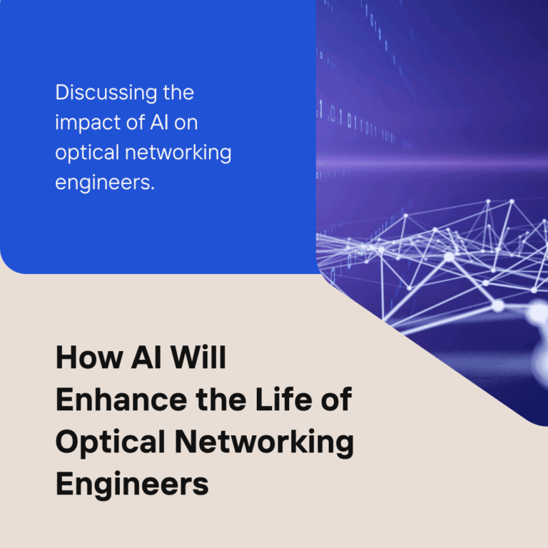
The integration of artificial intelligence (AI) into optical networking is set to dramatically transform offering numerous benefits for engineers at all levels of expertise. From automating routine tasks to enhancing network performance and reliability, AI promises to make the lives of optical networking engineers easier and more productive. Here’s a detailed look at how AI is transforming this industry.

AI-Optical
AI-Optical

Automation and Efficiency

One of the most significant ways AI is enhancing optical networking is through automation. Routine tasks such as network monitoring, fault detection, and performance optimization can be automated using AI algorithms. This allows engineers to focus on more complex and innovative aspects of network management. AI-driven automation tools can identify and predict network issues before they become critical, reducing downtime and maintenance costs.Companies like Cisco are implementing AIOps (Artificial Intelligence for IT Operations), which leverages machine learning to streamline IT operations. This involves using AI to analyse data from network devices, predict potential failures, and automate remediation processes. Such systems provide increased visibility into network operations, enabling quicker decision-making and problem resolution

Enhanced Network Performance

AI can significantly enhance network performance by optimising traffic flow and resource allocation. AI algorithms analyse vast amounts of data to understand network usage patterns and adjust resources dynamically. This leads to more efficient utilisation of bandwidth and improved overall network performance​ . Advanced AI models can predict traffic congestion and reroute data to prevent bottlenecks. For instance, in data centers where AI and machine learning workloads are prevalent, AI can manage data flow to ensure that high-priority tasks receive the necessary bandwidth, thereby improving processing efficiency and reducing latency​

Predictive Maintenance

AI’s predictive capabilities are invaluable in maintaining optical networks. By analysing historical data and identifying patterns, AI can predict when and where equipment failures are likely to occur. This proactive approach allows for maintenance to be scheduled during non-peak times, minimising disruption to services​ Using AI, engineers can monitor the health of optical transceivers and other critical components in real-time. Predictive analytics can forecast potential failures, enabling preemptive replacement of components before they fail, thus ensuring continuous network availability​ .

Improved Security

AI enhances the security of optical networks by detecting and mitigating threats in real-time. Machine learning algorithms can identify unusual network behavior that may indicate a security breach, allowing for immediate response to potential threats​.AI-driven security systems can analyse network traffic to identify patterns indicative of cyber-attacks. These systems can automatically implement countermeasures to protect the network, significantly reducing the risk of data breaches and other security incidents​.

Bridging the Skills Gap

For aspiring optical engineers, AI can serve as a powerful educational tool. AI-powered simulation and training programs can provide hands-on experience with network design, deployment, and troubleshooting. This helps bridge the skills gap and prepares new engineers to handle complex optical networking tasks​ Educational institutions and training providers are leveraging AI to create immersive learning environments. These platforms can simulate real-world network scenarios, allowing students to practice and hone their skills in a controlled setting before applying them in the field​ .

Future Trends

Looking ahead, the role of AI in optical networking will continue to expand. Innovations such as 800G pluggables and 1.6T coherent optical engines are on the horizon, promising to push network capacity to new heights. As optical networking technology continues to advance, AI will play an increasingly central role. From managing ever-growing data flows to ensuring the highest levels of network security, AI tools offer unprecedented advantages. The integration of AI into optical networking promises not only to improve the quality of network services but also to redefine the role of the network engineer. With AI’s potential still unfolding, the future holds exciting prospects for innovation and efficiency in optical networking.

References:

The advent of 5G technology is set to revolutionise the way we connect, and at its core lies a sophisticated transport network architecture. This architecture is designed to support the varied requirements of 5G’s advanced services and applications.

As we migrate from the legacy 4G to the versatile 5G, the transport network must evolve to accommodate new deployment strategies influenced by the functional split options specified by 3GPP and the drift of the Next Generation Core (NGC) network towards cloud-edge deployment.

5G
Deployment location of core network in 5G network

The Four Pillars of 5G Transport Network

1. Fronthaul: This segment of the network deals with the connection between the high PHY and low PHY layers. It requires a high bandwidth, about 25 Gbit/s for a single UNI interface, escalating to 75 or 150 Gbit/s for an NNI interface in pure 5G networks. In hybrid 4G and 5G networks, this bandwidth further increases. The fronthaul’s stringent latency requirements (<100 microseconds) necessitate point-to-point (P2P) deployment to ensure rapid and efficient data transfer.

2. Midhaul: Positioned between the Packet Data Convergence Protocol (PDCP) and Radio Link Control (RLC), the midhaul section plays a pivotal role in data aggregation. Its bandwidth demands are slightly less than that of the fronthaul, with UNI interfaces handling 10 or 25 Gbit/s and NNI interfaces scaling according to the DU’s aggregation capabilities. The midhaul network typically adopts tree or ring modes to efficiently connect multiple Distributed Units (DUs) to a centralized Control Unit (CU).

3. Backhaul: Above the Radio Resource Control (RRC), the backhaul shares similar bandwidth needs with the midhaul. It handles both horizontal traffic, coordinating services between base stations, and vertical traffic, funneling various services like Vehicle to Everything (V2X), enhanced Mobile BroadBand (eMBB), and Internet of Things (IoT) from base stations to the 5G core.

4. NGC Interconnection: This crucial juncture interconnects nodes post-deployment in the cloud edge, demanding bandwidths equal to or in excess of 100 Gbit/s. The architecture aims to minimize bandwidth wastage, which is often a consequence of multi-hop connections, by promoting single hop connections.

The Impact of Deployment Locations

The transport network’s deployment locations—fronthaul, midhaul, backhaul, and NGC interconnection—each serve unique functions tailored to the specific demands of 5G services. From ensuring ultra-low latency in fronthaul to managing service diversity in backhaul, and finally facilitating high-capacity connectivity in NGC interconnections, the transport network is the backbone that supports the high-speed, high-reliability promise of 5G.

As we move forward into the 5G era, understanding and optimizing these transport network segments will be crucial for service providers to deliver on the potential of this transformative technology.

Reference

https://www.itu.int/rec/T-REC-G.Sup67-201907-I/en

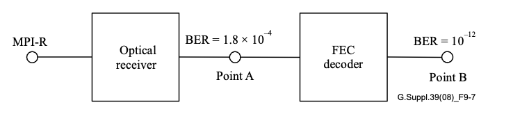
Forward Error Correction (FEC) has become an indispensable tool in modern optical communication, enhancing signal integrity and extending transmission distances. ITU-T recommendations, such as G.693, G.959.1, and G.698.1, define application codes for optical interfaces that incorporate FEC as specified in ITU-T G.709. In this blog, we discuss the significance of Bit Error Ratio (BER) in FEC-enabled applications and how it influences optical transmitter and receiver performance.

The Basics of FEC in Optical Communications

FEC is a method of error control for data transmission, where the sender adds redundant data to its messages. This allows the receiver to detect and correct errors without the need for retransmission. In the context of optical networks, FEC is particularly valuable because it can significantly lower the BER after decoding, thus ensuring the accuracy and reliability of data across vast distances.

BER Requirements in FEC-Enabled Applications

For certain optical transport unit rates (OTUk), the system BER is mandated to meet specific standards only after FEC correction has been applied. The optical parameters, in these scenarios, are designed to achieve a BER no worse than 10−12 at the FEC decoder’s output. This benchmark ensures that the data, once processed by the FEC decoder, maintains an extremely high level of accuracy, which is crucial for high-performance networks.

Practical Implications for Network Hardware

When it comes to testing and verifying the performance of optical hardware components intended for FEC-enabled applications, achieving a BER of 10−12 at the decoder’s output is often sufficient. Attempting to test components at 10−12 at the receiver output, prior to FEC decoding, can lead to unnecessarily stringent criteria that may not reflect the operational requirements of the application.

Adopting Appropriate BER Values for Testing

The selection of an appropriate BER for testing components depends on the specific application. Theoretical calculations suggest a BER of 1.8×10⁻⁴at the receiver output (Point A) to achieve a BER of 10−12 at the FEC decoder output (Point B). However, due to variations in error statistics, the average BER at Point A may need to be lower than the theoretical value to ensure the desired BER at Point B. In practice, a BER range of 10−5 to 10−6 is considered suitable for most applications.

Conservative Estimation for Receiver Sensitivity

By using a BER of 10−6 for component verification, the measurements of receiver sensitivity and optical path penalty at Point A will be conservative estimates of the values after FEC correction. This approach provides a practical and cost-effective method for ensuring component performance aligns with the rigorous demands of FEC-enabled systems.

Conclusion

FEC is a powerful mechanism that significantly improves the error tolerance of optical communication systems. By understanding and implementing appropriate BER testing methodologies, network operators can ensure their components are up to the task, ultimately leading to more reliable and efficient networks.

As the demands for data grow, the reliance on sophisticated FEC techniques will only increase, cementing BER as a fundamental metric in the design and evaluation of optical communication systems.

References

https://www.itu.int/rec/T-REC-G/e

When we talk about the internet and data, what often comes to mind are the speeds and how quickly we can download or upload content. But behind the scenes, it’s a game of efficiently packing data signals onto light waves traveling through optical fibers.If you’re an aspiring telecommunications professional or a student diving into the world of fiber optics, understanding the allocation of spectral bands is crucial. It’s like knowing the different climates in a world map of data transmission. Let’s explore the significance of these bands as defined by ITU-T recommendations and what they mean for fiber systems.

#opticalband

The Role of Spectral Bands in Single-Mode Fiber Systems

Original O-Band (1260 – 1360 nm): The journey of fiber optics began with the O-band, chosen for ITU T G.652 fibers due to its favorable dispersion characteristics and alignment with the cut-off wavelength of the cable. This band laid the groundwork for optical transmission without the need for amplifiers, making it a cornerstone in the early days of passive optical networks.

Extended E-Band (1360 – 1460 nm): With advancements, the E-band emerged to accommodate the wavelength drift of uncooled lasers. This extended range allowed for greater flexibility in transmissions, akin to broadening the canvas on which network artists could paint their data streams.

Short Wavelength S-Band (1460 – 1530 nm): The S-band, filling the gap between the E and C bands, has historically been underused for data transmission. However, it plays a crucial role in supporting the network infrastructure by housing pump lasers and supervisory channels, making it the unsung hero of the optical spectrum.

Conventional C-Band (1530 – 1565 nm): The beloved C-band owes its popularity to the era of erbium-doped fiber amplifiers (EDFAs), which provided the necessary gain for dense wavelength division multiplexing (DWDM) systems. It’s the bread and butter of the industry, enabling vast data capacity and robust long-haul transmissions.

Long Wavelength L-Band (1565 – 1625 nm): As we seek to expand our data highways, the L-band has become increasingly important. With fiber performance improving over a range of temperatures, this band offers a wider wavelength range for signal transmission, potentially doubling the capacity when combined with the C-band.

Ultra-Long Wavelength U-Band (1625 – 1675 nm): The U-band is designated mainly for maintenance purposes and is not currently intended for transmitting traffic-bearing signals. This band ensures the network’s longevity and integrity, providing a dedicated spectrum for testing and monitoring without disturbing active data channels.

Historical Context and Technological Progress

It’s fascinating to explore why we have bands at all. The ITU G-series documents paint a rich history of fiber deployment, tracing the evolution from the first multimode fibers to the sophisticated single-mode fibers we use today.

In the late 1970s, multimode fibers were limited by both high attenuation at the 850 nm wavelength and modal dispersion. A leap to 1300 nm in the early 1980s marked a significant drop in attenuation and the advent of single-mode fibers. By the late 1980s, single-mode fibers were achieving commercial transmission rates of up to 1.7 Gb/s, a stark contrast to the multimode fibers of the past.

The designation of bands was a natural progression as single-mode fibers were designed with specific cutoff wavelengths to avoid modal dispersion and to capitalize on the low attenuation properties of the fiber.

The Future Beckons

With the ITU T G.65x series recommendations setting the stage, we anticipate future applications utilizing the full spectrum from 1260 nm to 1625 nm. This evolution, coupled with the development of new amplification technologies like thulium-doped amplifiers or Raman amplification, suggests that the S-band could soon be as important as the C and L bands.

Imagine a future where the combination of S+C+L bands could triple the capacity of our fiber infrastructure. This isn’t just a dream; it’s a realistic projection of where the industry is headed.

Conclusion

The spectral bands in fiber optics are not just arbitrary divisions; they’re the result of decades of research, development, and innovation. As we look to the horizon, the possibilities are as wide as the spectrum itself, promising to keep pace with our ever-growing data needs.

Reference

https://www.itu.int/rec/T-REC-G/e