Exploring the C+L Bands in DWDM Network

https://www.itu.int/rec/T-REC-G.Sup67/en

As the 5G era dawns, the need for robust transport network architectures has never been more critical. The advent of 5G brings with it a promise of unprecedented data speeds and connectivity, necessitating a backbone capable of supporting a vast array of services and applications. In this realm, the Optical Transport Network (OTN) emerges as a key player, engineered to meet the demanding specifications of 5G’s advanced network infrastructure.

Understanding OTN’s Role

The 5G transport network is a multifaceted structure, composed of fronthaul, midhaul, and backhaul components, each serving a unique function within the overarching network ecosystem. Adaptability is the name of the game, with various operators customizing their network deployment to align with individual use cases as outlined by the 3rd Generation Partnership Project (3GPP).

C-RAN: Centralized Radio Access Network

In the C-RAN scenario, the Active Antenna Unit (AAU) is distinct from the Distribution Unit (DU), with the DU and Central Unit (CU) potentially sharing a location. This configuration leads to the presence of fronthaul and backhaul networks, and possibly midhaul networks. The fronthaul segment, in particular, is characterized by higher bandwidth demands, catering to the advanced capabilities of technologies like enhanced Common Public Radio Interface (eCPRI).

C-RAN Deployment Specifics:

Large C-RAN: DUs are centrally deployed at the central office (CO), which typically is the intersection point of metro-edge fibre rings. The number of DUs within in each CO is between 20 and 60 (assume each DU is connected to 3 AAUs).
Small C-RAN: DUs are centrally deployed at the metro-edge site, which typically is located at the metro-edge fibre ring handover point. The number of DUs within each metro-edge site is around 5~10

D-RAN: Distributed Radio Access Network

The D-RAN setup co-locates the AAU with the DU, eliminating the need for a dedicated fronthaul network. This streamlined approach focuses on backhaul (and potentially midhaul) networks, bypassing the fronthaul segment altogether.

5G transport network architecture: D-RAN

NGC: Next Generation Core Interconnection

The NGC interconnection serves as the network’s spine, supporting data transmission capacities ranging from 0.8 to 2 Tbit/s, with latency requirements as low as 1 ms, and reaching distances between 100 to 200 km.

Transport Network Requirement Summary for NGC:

Parameter	Requirement	Comments
Capacity	0.8-2 Tbit/s	Each NGC node has 500 base stations. The average bandwidth of each base station is about 3Gbit/s, the convergence ratio is 1/4, and the typical bandwidth of NGC nodes is about 400Gbit/s. 2~5 directions are considered, so the NGC node capacity is 0.8~2Tbit/s.
Latency	1 ms	Round trip time (RTT) latency between NGCs required for DC hot backup intra-city.
Reach	100-200 km	Typical distance between NGCs.

Note: These requirements will vary among network operators.

The Future of 5G Transport Networks

The blueprint for 5G networks is complex, yet it must ensure seamless service delivery. The diversity of OTN architectures, from C-RAN to D-RAN and the strategic NGC interconnections, underscores the flexibility and scalability essential for the future of mobile connectivity. As 5G unfolds, the ability of OTN architectures to adapt and scale will be pivotal in meeting the ever-evolving landscape of digital communication.

References

In Standards 3 Mins Read

Basics of 5G Transport Network Architecture

https://www.itu.int/rec/T-REC-G.Sup67-201907-I/en

The advent of 5G technology is set to revolutionise the way we connect, and at its core lies a sophisticated transport network architecture. This architecture is designed to support the varied requirements of 5G’s advanced services and applications.

As we migrate from the legacy 4G to the versatile 5G, the transport network must evolve to accommodate new deployment strategies influenced by the functional split options specified by 3GPP and the drift of the Next Generation Core (NGC) network towards cloud-edge deployment.

**Deployment location of core network in 5G network**

The Four Pillars of 5G Transport Network

1. Fronthaul: This segment of the network deals with the connection between the high PHY and low PHY layers. It requires a high bandwidth, about 25 Gbit/s for a single UNI interface, escalating to 75 or 150 Gbit/s for an NNI interface in pure 5G networks. In hybrid 4G and 5G networks, this bandwidth further increases. The fronthaul’s stringent latency requirements (<100 microseconds) necessitate point-to-point (P2P) deployment to ensure rapid and efficient data transfer.

2. Midhaul: Positioned between the Packet Data Convergence Protocol (PDCP) and Radio Link Control (RLC), the midhaul section plays a pivotal role in data aggregation. Its bandwidth demands are slightly less than that of the fronthaul, with UNI interfaces handling 10 or 25 Gbit/s and NNI interfaces scaling according to the DU’s aggregation capabilities. The midhaul network typically adopts tree or ring modes to efficiently connect multiple Distributed Units (DUs) to a centralized Control Unit (CU).

3. Backhaul: Above the Radio Resource Control (RRC), the backhaul shares similar bandwidth needs with the midhaul. It handles both horizontal traffic, coordinating services between base stations, and vertical traffic, funneling various services like Vehicle to Everything (V2X), enhanced Mobile BroadBand (eMBB), and Internet of Things (IoT) from base stations to the 5G core.

4. NGC Interconnection: This crucial juncture interconnects nodes post-deployment in the cloud edge, demanding bandwidths equal to or in excess of 100 Gbit/s. The architecture aims to minimize bandwidth wastage, which is often a consequence of multi-hop connections, by promoting single hop connections.

The Impact of Deployment Locations

The transport network’s deployment locations—fronthaul, midhaul, backhaul, and NGC interconnection—each serve unique functions tailored to the specific demands of 5G services. From ensuring ultra-low latency in fronthaul to managing service diversity in backhaul, and finally facilitating high-capacity connectivity in NGC interconnections, the transport network is the backbone that supports the high-speed, high-reliability promise of 5G.

As we move forward into the 5G era, understanding and optimizing these transport network segments will be crucial for service providers to deliver on the potential of this transformative technology.

Reference

In Standards 4 Mins Read

OTN Secure Transport

https://www.itu.int/rec/T-REC-G.Sup76/en

In today’s world, where digital information rules, keeping networks secure is not just important—it’s essential for the smooth operation of all our communication systems. Optical Transport Networking (OTN), which follows rules set by standards like ITU-T G.709 and ITU-T G.709.1, is leading the charge in making sure data gets where it’s going safely. This guide takes you through the essentials of OTN secure transport, highlighting how encryption and authentication are key to protecting sensitive data as it moves across networks.

The Introduction of OTN Security

Layer 1 encryption, or OTN security (OTNsec), is not just a feature—it’s a fundamental aspect that ensures the safety of data as it traverses the complex web of modern networks. Recognized as a market imperative, OTNsec provides encryption at the physical layer, thwarting various threats such as control management breaches, denial of service attacks, and unauthorized access.

Conceptualizing Secure Transport

OTN secure transport can be visualized through two conceptual approaches. The first, and the primary focus of this guide, involves the service requestor deploying endpoints within its domain to interface with an untrusted domain. The second approach sees the service provider offering security endpoints and control over security parameters, including key management and agreement, to the service requestor.

OTN Security Applications

As network operators and service providers grapple with the need for data confidentiality and authenticity, OTN emerges as a robust solution. From client end-to-end security to service provider path end-to-end security, OTN’s applications are diverse.

Client End-to-End Security

This suite of applications ensures that the operator’s OTN network remains oblivious to the client layer security, which is managed entirely within the customer’s domain. Technologies such as MACsec [IEEE 802.1AE] for Ethernet clients provide encryption and authentication at the client level.Following are some of the scenerios.

Client end-to-end security (with CPE)

Client end-to-end security (without CPE)

DC, content or mobile service provider client end-to-end security

Service Provider CPE End-to-End Security

Service providers can offer security within the OTN service of the operator’s network. This scenario sees the service provider managing key agreements, with the UNI access link being the only unprotected element, albeit within the trusted customer premises.

Service provider CPE end-to-end security

OTN Link/Span Security

Operators can fortify their network infrastructure using encryption and authentication on a per-span basis. This is particularly critical when the links interconnect various OTN network elements within the same administrative domain.

Second Operator and Access Link Security

When services traverse the networks of multiple operators, securing each link becomes paramount. Whether through client access link security or OTN service provider access link security, OTN facilitates a protected handoff between customer premises and the operator.

Multi-Layered Security in OTN

OTN’s versatility allows for multi-layered security, combining protocols that offer different characteristics and serve complementary functions. From end-to-end encryption at the client layer to additional encryption at the ODU layer, OTN accommodates various security needs without compromising on performance.

Final Observations

OTN security applications must ensure transparency across network elements not participating as security endpoints. Support for multiple levels of ODUj to ODUk schemes, interoperable cipher suite types for PHY level security, and the ability to handle subnetworks and TCMs are all integral to OTN’s security paradigm.

This blog provides a detailed exploration of OTN secure transport, encapsulating the strategic implementation of security measures in optical networks. It underscores the importance of encryption and authentication in maintaining data integrity and confidentiality, positioning OTN as a critical component in the infrastructure of secure communication networks.

By adhering to these security best practices, network operators can not only safeguard their data but also enhance the overall trust in their communication systems, paving the way for a secure and reliable digital future.

References

More Detail article can be read on ITU-T at

In Standards 6 Mins Read

Comprehensive Guide to Optical Power Safety in Fiber Optic Communications

Fiber optics has revolutionized the way we transmit data, offering faster speeds and higher capacity than ever before. However, as with any powerful technology, there are significant safety considerations that must be taken into account to protect both personnel and equipment. This comprehensive guide provides an in-depth look at best practices for optical power safety in fiber optic communications.

Viewing Safety Measures

Directly viewing fiber ends or connector faces can be hazardous. It’s crucial to use only approved filtered or attenuating viewing aids to inspect these components. This protects the eyes from potentially harmful laser emissions that can cause irreversible damage.

Fiber End Management

Unterminated fiber ends, if left uncovered, can emit laser light that is not only a safety hazard but can also compromise the integrity of the optical system. When fibers are not being actively used, they should be covered with material suitable for the specific wavelength and power, such as a splice protector or tape. This precaution ensures that sharp ends are not exposed, and the fiber ends are not readily visible, minimizing the risk of accidental exposure.

The Crucial Role of Cleaning

Optical connectors must be kept clean, especially in high-power systems. Contaminants can lead to the fiber-fuse phenomenon, where high temperatures and bright white light propagate down the fiber, creating a safety hazard. Before any power is applied, ensure that all fiber ends are free from contaminants.

Managing Connector and Splice Loss

Even a small amount of loss at connectors or splices can lead to a significant increase in temperature, particularly in high-power systems. Choosing the right connectors and managing splices carefully can prevent local heating that might otherwise escalate to system damage.

Ribbon Fibers and Test Cords

Ribbon fibers, when cleaved as a unit, can present a higher hazard level than single fibers. They should not be cleaved or spliced as an unseparated ribbon unless explicitly authorized. When using optical test cords, always connect the optical power source last and disconnect it first to avoid any inadvertent exposure to active laser light.

Avoiding Excessive Bending

Fiber optics are delicate and can be damaged by excessive bending, which not only risks mechanical failure but also creates potential hotspots in high-power transmission. Careful routing and handling of fibers to avoid low-radius bends are essential best practices.

Handling Board Extenders and Routine Maintenance

Board extenders should never be used with optical transmitter or amplifier cards. Only perform maintenance tasks in accordance with the procedures approved by the operating organization to avoid unintended system alterations that could lead to safety issues.

Test Equipment Usage

Employ test equipment that is appropriate for the task at hand. Using equipment with a power rating higher than necessary can introduce unnecessary risk. Ensure that the class of the test equipment matches the hazard level of the location where it’s being used.

System Modifications and Key Control

Unauthorized modifications to optical fiber communication systems or related equipment are strictly prohibited, as they can introduce unforeseen hazards. Additionally, key control for equipment should be managed by a responsible individual to ensure the safe and proper use of all devices.

Labeling and Signage

Optical safety labels are a critical aspect of safety. Any damaged or missing labels should be reported immediately. Warning signs should be posted in areas exceeding hazard level 1M, and even in lower classification locations, signs can provide an additional layer of safety.

Alarm Systems

Pay close attention to system alarms, particularly those indicating issues with automatic power reduction (APR) or other safety mechanisms. Prompt response to alarms can prevent minor issues from escalating into major safety concerns.

Raman Amplified Systems: A Special Note

Raman amplified systems operate at sufficiently high powers that can cause damage to fibre or other components. This is somewhat described in clauses 14.2 and 14.5, but some additional guidance follows:

Before activating the Raman power

– Calculate the distance to where the power is reduced to less than 150 mW.

– If possible, inspect any splicing enclosures within that distance. If tight bends, e.g., less than 20mm diameter, are seen, try to remove or relieve the bend, or choose other fibres.

– If inspection is not possible, a high resolution OTDR might be used to identify sources of bend or connector loss that could lead to damage under high power.

– If connectors are used, it should be verified that the ends are very clean. Metallic contaminants are particularly prone to causing damage. Fusion splices are considered to be the least subject to damage.

While activating Raman power

In some cases, it may be possible to monitor the reflected light at the source as the Raman pump power is increased. If the plot of reflected power versus injected power shows a non‑linear characteristic, there could be a reflective site that is subject to damage. Other sites subject to damage, such as tight bends in which the coating absorbs the optical power, may be present without showing a clear signal in the reflected power versus injected power curve.

Operating considerations

If there is a reduction in the amplification level over time, it could be due to a reduced pump power or due to a loss increase induced by some slow damage mechanism such as at a connector interface. Simply increasing the pump power to restore the signal could lead to even more damage or catastrophic failure.

The mechanism for fibre failure in bending is that light escapes from the cladding and some is absorbed by the coating, which results in local heating and thermal reactions. These reactions tend to increase the absorption and thus increase the heating. When a carbon layer is formed, there is a runaway thermal reaction that produces enough heat to melt the fibre, which then goes into a kinked state that blocks all optical power. Thus, there will be very little change in the transmission characteristics induced by a damaging process until the actual failure occurs. If the fibre is unbuffered, there is a flash at the moment of failure which is self-extinguishing because the coating is gone very quickly. A buffered fibre could produce more flames, depending on the material. For unbuffered fibre, sub-critical damage is evidenced by a colouring of the coating at the apex of the bend.

Conclusion

By following these best practices for optical power safety, professionals working with fiber optic systems can ensure a safe working environment while maintaining the integrity and performance of the communication systems they manage.

For those tasked with the maintenance and operation of fiber optic systems, this guide serves as a critical resource, outlining the necessary precautions to ensure safety in the workplace. As the technology evolves, so too must our commitment to maintaining stringent safety standards in the dynamic field of fiber optic communications.

References

In Standards 4 Mins Read

FEC in Optical Transmission Systems

In the pursuit of ever-greater data transmission capabilities, forward error correction (FEC) has emerged as a pivotal technology, not just in wireless communication but increasingly in large-capacity, long-haul optical systems. This blog post delves into the intricacies of FEC and its profound impact on the efficiency and cost-effectiveness of modern optical networks.

The Introduction of FEC in Optical Communications

FEC’s principle is simple yet powerful: by encoding the original digital signal with additional redundant bits, it can correct errors that occur during transmission. This technique enables optical transmission systems to tolerate much higher bit error ratios (BERs) than the traditional threshold of 10−1210−12 before decoding. Such resilience is revolutionizing system design, allowing the relaxation of optical parameters and fostering the development of vast, robust networks.

Defining FEC: A Glossary of Terms

Understanding FEC starts with grasping its key terminology. Here’s a brief rundown:

Information bit (byte): The original digital signal that will be encoded using FEC before transmission.
FEC parity bit (byte): Redundant data added to the original signal for error correction purposes.
Code word: A combination of information and FEC parity bits.
Code rate (R): The ratio of the original bit rate to the bit rate with FEC—indicative of the amount of redundancy added.
Coding gain: The improvement in signal quality as a result of FEC, quantified by a reduction in Q values for a specified BER.
Net coding gain (NCG): Coding gain adjusted for noise increase due to the additional bandwidth needed for FEC bits.

The Role of FEC in Optical Networks

The application of FEC allows for systems to operate with a BER that would have been unacceptable in the past, particularly in high-capacity, long-haul systems where the cumulative noise can significantly degrade signal quality. With FEC, these systems can achieve reliable performance even with the presence of amplified spontaneous emission (ASE) noise and other signal impairments.

In-Band vs. Out-of-Band FEC

There are two primary FEC schemes used in optical transmission: in-band and out-of-band FEC. In-band FEC, used in Synchronous Digital Hierarchy (SDH) systems, embeds FEC parity bits within the unused section overhead of SDH signals, thus not increasing the bit rate. In contrast, out-of-band FEC, as utilized in Optical Transport Networks (OTNs) and originally recommended for submarine systems, increases the line rate to accommodate FEC bits. ITU-T G.709 also introduces non-standard out-of-band FEC options optimized for higher efficiency.

Achieving Robustness Through FEC

The FEC schemes allow the correction of multiple bit errors, enhancing the robustness of the system. For example, a triple error-correcting binary BCH code can correct up to three bit errors in a 4359 bit code word, while an RS(255,239) code can correct up to eight byte errors per code word.

Performance of standard FECs

The Practical Impact of FEC

Implementing FEC leads to more forgiving system designs, where the requirement for pristine optical parameters is lessened. This, in turn, translates to reduced costs and complexity in constructing large-scale optical networks. The coding gains provided by FEC, especially when considered in terms of net coding gain, enable systems to better estimate and manage the OSNR, crucial for maintaining high-quality signal transmission.

Future Directions

While FEC has proven effective in OSNR-limited and dispersion-limited systems, its efficacy against phenomena like polarization mode dispersion (PMD) remains a topic for further research. Additionally, the interplay of FEC with non-linear effects in optical fibers, such as self-phase modulation and cross-phase modulation, presents a rich area for ongoing study.

Conclusion

FEC stands as a testament to the innovative spirit driving optical communications forward. By enabling systems to operate with higher BERs pre-decoding, FEC opens the door to more cost-effective, expansive, and resilient optical networks. As we look to the future, the continued evolution of FEC promises to underpin the next generation of optical transmission systems, making the dream of a hyper-connected world a reality.

References

In Standards 4 Mins Read

Noise Concatenation in Optical Amplifier Chains

Optical networks are the backbone of the internet, carrying vast amounts of data over great distances at the speed of light. However, maintaining signal quality over long fiber runs is a challenge due to a phenomenon known as noise concatenation. Let’s delve into how amplified spontaneous emission (ASE) noise affects Optical Signal-to-Noise Ratio (OSNR) and the performance of optical amplifier chains.

The Challenge of ASE Noise

ASE noise is an inherent byproduct of optical amplification, generated by the spontaneous emission of photons within an optical amplifier. As an optical signal traverses through a chain of amplifiers, ASE noise accumulates, degrading the OSNR with each subsequent amplifier in the chain. This degradation is a crucial consideration in designing long-haul optical transmission systems.

Understanding OSNR

OSNR measures the ratio of signal power to ASE noise power and is a critical parameter for assessing the performance of optical amplifiers. A high OSNR indicates a clean signal with low noise levels, which is vital for ensuring data integrity.

Reference System for OSNR Estimation

As depicted in Figure below), a typical multichannel N span system includes a booster amplifier, N−1 line amplifiers, and a preamplifier. To simplify the estimation of OSNR at the receiver’s input, we make a few assumptions:

Representation of optical line system interfaces (a multichannel N-span system)

All optical amplifiers, including the booster and preamplifier, have the same noise figure.
The losses of all spans are equal, and thus, the gain of the line amplifiers compensates exactly for the loss.
The output powers of the booster and line amplifiers are identical.

Estimating OSNR in a Cascaded System

E1: Master Equation For OSNR

P_out is the output power (per channel) of the booster and line amplifiers in dBm, L is the span loss in dB (which is assumed to be equal to the gain of the line amplifiers), G_BA is the gain of the optical booster amplifier in dB, NFis the signal-spontaneous noise figure of the optical amplifier in dB, h is Planck’s constant (in mJ·s to be consistent with P_out in dBm), ν is the optical frequency in Hz, ν_r is the reference bandwidth in Hz (corresponding to c/Br ), N–1 is the total number of line amplifiers.

The OSNR at the receivers can be approximated by considering the output power of the amplifiers, the span loss, the gain of the optical booster amplifier, and the noise figure of the amplifiers. Using constants such as Planck’s constant and the optical frequency, we can derive an equation that sums the ASE noise contributions from all N+1 amplifiers in the chain.

Simplifying the Equation

Under certain conditions, the OSNR equation can be simplified. If the booster amplifier’s gain is similar to that of the line amplifiers, or if the span loss greatly exceeds the booster gain, the equation can be modified to reflect these scenarios. These simplifications help network designers estimate OSNR without complex calculations.

1) If the gain of the booster amplifier is approximately the same as that of the line amplifiers, i.e., G_BA » L, above Equation E1 can be simplified to:

E1-1

2) The ASE noise from the booster amplifier can be ignored only if the span loss L (resp. the gain of the line amplifier) is much greater than the booster gain G_BA. In this case Equation E1-1 can be simplified to:

E1-2

3) Equation E1-1 is also valid in the case of a single span with only a booster amplifier, e.g., short‑haul multichannel IrDI in Figure 5-5 of [ITU-T G.959.1], in which case it can be modified to:

E1-3

4) In case of a single span with only a preamplifier, Equation E1 can be modified to:

Practical Implications for Network Design

Understanding the accumulation of ASE noise and its impact on OSNR is crucial for designing reliable optical networks. It informs decisions on amplifier placement, the necessity of signal regeneration, and the overall system architecture. For instance, in a system where the span loss is significantly high, the impact of the booster amplifier on ASE noise may be negligible, allowing for a different design approach.

Conclusion

Noise concatenation is a critical factor in the design and operation of optical networks. By accurately estimating and managing OSNR, network operators can ensure signal quality, minimize error rates, and extend the reach of their optical networks.

In a landscape where data demands are ever-increasing, mastering the intricacies of noise concatenation and OSNR is essential for anyone involved in the design and deployment of optical communication systems.

References

In Standards 3 Mins Read

BER and FEC in Optical Network Performance

Forward Error Correction (FEC) has become an indispensable tool in modern optical communication, enhancing signal integrity and extending transmission distances. ITU-T recommendations, such as G.693, G.959.1, and G.698.1, define application codes for optical interfaces that incorporate FEC as specified in ITU-T G.709. In this blog, we discuss the significance of Bit Error Ratio (BER) in FEC-enabled applications and how it influences optical transmitter and receiver performance.

The Basics of FEC in Optical Communications

FEC is a method of error control for data transmission, where the sender adds redundant data to its messages. This allows the receiver to detect and correct errors without the need for retransmission. In the context of optical networks, FEC is particularly valuable because it can significantly lower the BER after decoding, thus ensuring the accuracy and reliability of data across vast distances.

BER Requirements in FEC-Enabled Applications

For certain optical transport unit rates (OTUk), the system BER is mandated to meet specific standards only after FEC correction has been applied. The optical parameters, in these scenarios, are designed to achieve a BER no worse than 10⁻¹² at the FEC decoder’s output. This benchmark ensures that the data, once processed by the FEC decoder, maintains an extremely high level of accuracy, which is crucial for high-performance networks.

Practical Implications for Network Hardware

When it comes to testing and verifying the performance of optical hardware components intended for FEC-enabled applications, achieving a BER of 10⁻¹² at the decoder’s output is often sufficient. Attempting to test components at 10⁻¹² at the receiver output, prior to FEC decoding, can lead to unnecessarily stringent criteria that may not reflect the operational requirements of the application.

Adopting Appropriate BER Values for Testing

The selection of an appropriate BER for testing components depends on the specific application. Theoretical calculations suggest a BER of 1.8×10⁻⁴at the receiver output (Point A) to achieve a BER of 10⁻¹² at the FEC decoder output (Point B). However, due to variations in error statistics, the average BER at Point A may need to be lower than the theoretical value to ensure the desired BER at Point B. In practice, a BER range of 10⁻⁵ to 10⁻⁶ is considered suitable for most applications.

Conservative Estimation for Receiver Sensitivity

By using a BER of 10⁻⁶ for component verification, the measurements of receiver sensitivity and optical path penalty at Point A will be conservative estimates of the values after FEC correction. This approach provides a practical and cost-effective method for ensuring component performance aligns with the rigorous demands of FEC-enabled systems.

Conclusion

FEC is a powerful mechanism that significantly improves the error tolerance of optical communication systems. By understanding and implementing appropriate BER testing methodologies, network operators can ensure their components are up to the task, ultimately leading to more reliable and efficient networks.

As the demands for data grow, the reliance on sophisticated FEC techniques will only increase, cementing BER as a fundamental metric in the design and evaluation of optical communication systems.

References

In Standards 3 Mins Read

BER and Q Factor

Signal integrity is the cornerstone of effective fiber optic communication. In this sphere, two metrics stand paramount: Bit Error Ratio (BER) and Q factor. These indicators help engineers assess the performance of optical networks and ensure the fidelity of data transmission. But what do these terms mean, and how are they calculated?

What is BER?

BER represents the fraction of bits that have errors relative to the total number of bits sent in a transmission. It’s a direct indicator of the health of a communication link. The lower the BER, the more accurate and reliable the system.

ITU-T Standards Define BER Objectives

The ITU-T has set forth recommendations such as G.691, G.692, and G.959.1, which outline design objectives for optical systems, aiming for a BER no worse than 10⁻¹² at the end of a system’s life. This is a rigorous standard that guarantees high reliability, crucial for SDH and OTN applications.

Measuring BER

Measuring BER, especially as low as 10⁻¹², can be daunting due to the sheer volume of bits required to be tested. For instance, to confirm with 95% confidence that a system meets a BER of 10⁻¹², one would need to test 3×10¹² bits without encountering an error — a process that could take a prohibitively long time at lower transmission rates.

The Q Factor

The Q factor measures the signal-to-noise ratio at the decision point in a receiver’s circuitry. A higher Q factor translates to better signal quality. For a BER of 10⁻¹², a Q factor of approximately 7.03 is needed. The relationship between Q factor and BER, when the threshold is optimally set, is given by the following equations:

The general formula relating Q to BER is:

A common approximation for high Q values is:

For a more accurate calculation across the entire range of Q, the formula is:

Practical Example: Calculating BER from Q Factor

Let’s consider a practical example. If a system’s Q factor is measured at 7, what would be the approximate BER?

Using the approximation formula, we plug in the Q factor:

This would give us an approximate BER that’s indicative of a highly reliable system. For exact calculations, one would integrate the Gaussian error function as described in the more detailed equations.

Graphical Representation

The graph typically illustrates these relationships, providing a visual representation of how the BER changes as the Q factor increases. This allows engineers to quickly assess the signal quality without long, drawn-out error measurements.

Concluding Thoughts

Understanding and applying BER and Q factor calculations is crucial for designing and maintaining robust optical communication systems. These concepts are not just academic; they directly impact the efficiency and reliability of the networks that underpin our modern digital world.

References

In Standards 3 Mins Read

Spectral Bands for Multi Mode Optical Fiber Systems

While single-mode fibers have been the mainstay for long-haul telecommunications, multimode fibers hold their own, especially in applications where short distance and high bandwidth are critical. Unlike their single-mode counterparts, multimode fibers are not restricted by cut-off wavelength considerations, offering unique advantages.

The Nature of Multimode Fibers

Multimode fibers, characterized by a larger core diameter compared to single-mode fibers, allow multiple light modes to propagate simultaneously. This results in modal dispersion, which can limit the distance over which the fiber can operate without significant signal degradation. However, multimode fibers exhibit greater tolerance to bending effects and typically showcase higher attenuation coefficients.

Wavelength Windows for Multimode Applications

Multimode fibers shine in certain “windows,” or wavelength ranges, which are optimized for specific applications and classifications. These windows are where the fiber performs best in terms of attenuation and bandwidth.

IEEE Serial Bus (around 850 nm): Typically used in consumer electronics, the 830-860 nm window is optimal for IEEE 1394 (FireWire) connections, offering high-speed data transfer over relatively short distances.

Fiber Channel (around 770-860 nm): For high-speed data transfer networks, such as those used in storage area networks (SANs), the 770-860 nm window is often used, although it’s worth noting that some applications may use single-mode fibers.

Ethernet Variants:

10BASE (800-910 nm): These standards define Ethernet implementations for local area networks, with 10BASE-F, -FB, -FL, and -FP operating within the 800-910 nm range.
100BASE-FX (1270-1380 nm) and FDDI (Fiber Distributed Data Interface): Designed for local area networks, they utilize a wavelength window around 1300 nm, where multimode fibers offer reliable performance for data transmission.
1000BASE-SX (770-860 nm) for Gigabit Ethernet (GbE): Optimized for high-speed Ethernet over multimode fiber, this application takes advantage of the lower window around 850 nm.
1000BASE-LX (1270-1355 nm) for GbE: This standard extends the use of multimode fibers into the 1300 nm window for Gigabit Ethernet applications.

HIPPI (High-Performance Parallel Interface): This high-speed computer bus architecture utilizes both the 850 nm and the 1300 nm windows, spanning from 830-860 nm and 1260-1360 nm, respectively, to support fast data transfers over multimode fibers.

Future Classifications and Studies

The classification of multimode fibers is a subject of ongoing research. Proposals suggest the use of the region from 770 nm to 910 nm, which could open up new avenues for multimode fiber applications. As technology progresses, these classifications will continue to evolve, reflecting the dynamic nature of fiber optic communications.

Wrapping Up: The Place of Multimode Fibers in Networking

Multimode fibers are a vital part of the networking world, particularly in scenarios that require high data rates over shorter distances. Their resilience to bending and capacity for high bandwidth make them an attractive choice for a variety of applications, from high-speed data transfer in industrial settings to backbone cabling in data centers.

As we continue to study and refine the classifications of multimode fibers, their role in the future of networking is guaranteed to expand, bringing new possibilities to the realm of optical communications.

References

In Standards 4 Mins Read

Spectral Bands for Single Mode Optical Fiber Systems

When we talk about the internet and data, what often comes to mind are the speeds and how quickly we can download or upload content. But behind the scenes, it’s a game of efficiently packing data signals onto light waves traveling through optical fibers.If you’re an aspiring telecommunications professional or a student diving into the world of fiber optics, understanding the allocation of spectral bands is crucial. It’s like knowing the different climates in a world map of data transmission. Let’s explore the significance of these bands as defined by ITU-T recommendations and what they mean for fiber systems.

The Role of Spectral Bands in Single-Mode Fiber Systems

Original O-Band (1260 – 1360 nm): The journey of fiber optics began with the O-band, chosen for ITU T G.652 fibers due to its favorable dispersion characteristics and alignment with the cut-off wavelength of the cable. This band laid the groundwork for optical transmission without the need for amplifiers, making it a cornerstone in the early days of passive optical networks.

Extended E-Band (1360 – 1460 nm): With advancements, the E-band emerged to accommodate the wavelength drift of uncooled lasers. This extended range allowed for greater flexibility in transmissions, akin to broadening the canvas on which network artists could paint their data streams.

Short Wavelength S-Band (1460 – 1530 nm): The S-band, filling the gap between the E and C bands, has historically been underused for data transmission. However, it plays a crucial role in supporting the network infrastructure by housing pump lasers and supervisory channels, making it the unsung hero of the optical spectrum.

Conventional C-Band (1530 – 1565 nm): The beloved C-band owes its popularity to the era of erbium-doped fiber amplifiers (EDFAs), which provided the necessary gain for dense wavelength division multiplexing (DWDM) systems. It’s the bread and butter of the industry, enabling vast data capacity and robust long-haul transmissions.

Long Wavelength L-Band (1565 – 1625 nm): As we seek to expand our data highways, the L-band has become increasingly important. With fiber performance improving over a range of temperatures, this band offers a wider wavelength range for signal transmission, potentially doubling the capacity when combined with the C-band.

Ultra-Long Wavelength U-Band (1625 – 1675 nm): The U-band is designated mainly for maintenance purposes and is not currently intended for transmitting traffic-bearing signals. This band ensures the network’s longevity and integrity, providing a dedicated spectrum for testing and monitoring without disturbing active data channels.

Historical Context and Technological Progress

It’s fascinating to explore why we have bands at all. The ITU G-series documents paint a rich history of fiber deployment, tracing the evolution from the first multimode fibers to the sophisticated single-mode fibers we use today.

In the late 1970s, multimode fibers were limited by both high attenuation at the 850 nm wavelength and modal dispersion. A leap to 1300 nm in the early 1980s marked a significant drop in attenuation and the advent of single-mode fibers. By the late 1980s, single-mode fibers were achieving commercial transmission rates of up to 1.7 Gb/s, a stark contrast to the multimode fibers of the past.

The designation of bands was a natural progression as single-mode fibers were designed with specific cutoff wavelengths to avoid modal dispersion and to capitalize on the low attenuation properties of the fiber.

The Future Beckons

With the ITU T G.65x series recommendations setting the stage, we anticipate future applications utilizing the full spectrum from 1260 nm to 1625 nm. This evolution, coupled with the development of new amplification technologies like thulium-doped amplifiers or Raman amplification, suggests that the S-band could soon be as important as the C and L bands.

Imagine a future where the combination of S+C+L bands could triple the capacity of our fiber infrastructure. This isn’t just a dream; it’s a realistic projection of where the industry is headed.

Conclusion

The spectral bands in fiber optics are not just arbitrary divisions; they’re the result of decades of research, development, and innovation. As we look to the horizon, the possibilities are as wide as the spectrum itself, promising to keep pace with our ever-growing data needs.

Reference

In Technical 2 Mins Read

Spectral Grids and WDM Techniques for Fiber Optic Capacity

Introduction

The telecommunications industry constantly strives to maximize the use of fiber optic capacity. Despite the broad spectral width of the conventional C-band, which offers over 40 THz, the limited use of optical channels at 10 or 40 Gbit/s results in substantial under utilization. The solution lies in Wavelength Division Multiplexing (WDM), a technique that can significantly increase the capacity of optical fibers.

Understanding Spectral Grids

WDM employs multiple optical carriers, each on a different wavelength, to transmit data simultaneously over a single fiber. This method vastly improves the efficiency of data transmission, as outlined in ITU-T Recommendations that define the spectral grids for WDM applications.

The Evolution of Channel Spacing

Historically, WDM systems have evolved to support an array of channel spacings. Initially, a 100 GHz grid was established, which was then subdivided by factors of two to create a variety of frequency grids, including:

12.5 GHz spacing
25 GHz spacing
50 GHz spacing
100 GHz spacing

All four frequency grids incorporate 193.1 THz and are not limited by frequency boundaries. Additionally, wider spacing grids can be achieved by using multiples of 100 GHz, such as 200 GHz, 300 GHz, and so on.

ITU-T Recommendations for DWDM

ITU-T Recommendations such as ITU-T G.692 and G.698 series outline applications utilizing these DWDM frequency grids. The recent addition of a flexible DWDM grid, as per Recommendation ITU-T G.694.1, allows for variable bit rates and modulation formats, optimizing the allocation of frequency slots to match specific bandwidth requirements.

Flexible DWDM Grid in Practice

The flexible grid is particularly innovative, with nominal central frequencies at intervals of 6.25 GHz from 193.1 THz and slot widths based on 12.5 GHz increments. This flexibility ensures that the grid can adapt to a variety of transmission needs without overlap, as depicted in Figure above.

CWDM Wavelength Grid and Applications

Recommendation ITU-T G.694.2 defines the CWDM wavelength grid to support applications requiring simultaneous transmission of several wavelengths. The 20 nm channel spacing is a result of manufacturing tolerances, temperature variations, and the need for a guardband to use cost-effective filter technologies. These CWDM grids are further detailed in ITU-T G.695.

Conclusion

The strategic use of DWDM and CWDM grids, as defined by ITU-T Recommendations, is key to maximizing the capacity of fiber optic transmissions. With the introduction of flexible grids and ongoing advancements, we are witnessing a transformative period in fiber optic technology.

In Standards 3 Mins Read

Anatomy of Outdoor and Indoor Optical Fiber Cables

https://www.itu.int/rec/T-REC-G.Sup40-201810-I/en

The world of optical communication is intricate, with different cable types designed for specific environments and applications. Today, we’re diving into the structure of two common types of optical fiber cables, as depicted in Figure below, and summarising the findings from an appendix that examined their performance.

Figure

Cable A: The Stranded Loose Tube Outdoor Cable

Cable A represents a quintessential outdoor cable, built to withstand the elements and the rigors of outdoor installation. The cross-section of this cable reveals a complex structure designed for durability and performance:

Central Strength Member: At its core, the cable has a central strength member that provides mechanical stability and ensures the cable can endure the tensions of installation.
Tube Filling Gel: Surrounding the central strength member are buffer tubes secured with a tube filling gel, which protects the fibers from moisture and physical stress.
Loose Tubes: These tubes hold the optical fibers loosely, allowing for expansion and contraction due to temperature changes without stressing the fibers themselves.
Fibers: Each tube houses six fibers, comprising various types specified by the ITU-T, including G.652.D, G.654.E, G.655.D, G.657.A1, G.657.A2, and G.657.B3. This array of fibers ensures compatibility with different transmission standards and conditions.
Aluminium Tape and PE Sheath: The aluminum tape provides a barrier against electromagnetic interference, while the polyethylene (PE) sheath offers physical protection and resistance to environmental factors.

The stranded loose tube design is particularly suited for long-distance outdoor applications, providing a robust solution for optical networks that span vast geographical areas.

Cable B: The Tight Buffered Indoor Cable

Switching our focus to indoor applications, Cable B is engineered for the unique demands of indoor environments:

Tight Buffered Fibers: Unlike Cable A, this indoor cable features four tight buffered fibers, which are more protected from physical damage and easier to handle during installation.
Aramid Yarn: Known for its strength and resistance to heat, aramid yarn is used to reinforce the cable, providing additional protection and tensile strength.
PE Sheath: Similar to Cable A, a PE sheath encloses the structure, offering a layer of defense against indoor environmental factors.

Cable B contains two ITU-T G.652.D fibers and two ITU-T G.657.B3 fibers, allowing for a blend of standard single-mode performance with the high bend-resistance characteristic of G.657.B3 fibers, making it ideal for complex indoor routing.

Conclusion

The intricate designs of optical fiber cables are tailored to their application environments. Cable A is optimized for outdoor use with a structure that guards against environmental challenges and mechanical stresses, while Cable B is designed for indoor use, where flexibility and ease of handling are paramount. By understanding the components and capabilities of these cables, network designers and installers can make informed decisions to ensure reliable and efficient optical communication systems.

Reference

In Standards 3 Mins Read

ITU-T Recommendations for Optical Fibers and Cables

In the realm of telecommunications, the precision and reliability of optical fibers and cables are paramount. The International Telecommunication Union (ITU) plays a crucial role in this by providing a series of recommendations that serve as global standards. The ITU-T G.650.x and G.65x series of recommendations are especially significant for professionals in the field. In this article, we delve into these recommendations and their interrelationships, as illustrated in Figure 1 .

ITU-T G.650.x Series: Definitions and Test Methods

The ITU-T G.650.x series is foundational for understanding single-mode fibers and cables. ITU-T G.650.1 is the cornerstone, offering definitions and test methods for linear and deterministic parameters of single-mode fibers. This includes key measurements like attenuation and chromatic dispersion, which are critical for ensuring fiber performance over long distances.

Moving forward, ITU-T G.650.2 expands on the initial parameters by providing definitions and test methods for statistical and non-linear parameters. These are essential for predicting fiber behavior under varying signal powers and during different transmission phenomena.

For those involved in assessing installed fiber links, ITU-T G.650.3 offers valuable test methods. It’s tailored to the needs of field technicians and engineers who analyze the performance of installed single-mode fiber cable links, ensuring that they meet the necessary standards for data transmission.

ITU-T G.65x Series: Specifications for Fibers and Cables

The ITU-T G.65x series recommendations provide specifications for different types of optical fibers and cables. ITU-T G.651.1 targets the optical access network with specifications for 50/125 µm multimode fiber and cable, which are widely used in local area networks and data centers due to their ability to support high data rates over short distances.

The series then progresses through various single-mode fiber specifications:

ITU-T G.652: The standard single-mode fiber, suitable for a wide range of applications.
ITU-T G.653: Dispersion-shifted fibers optimized for minimizing chromatic dispersion.
ITU-T G.654: Features a cut-off shifted fiber, often used for submarine cable systems.
ITU-T G.655: Non-zero dispersion-shifted fibers, which are ideal for long-haul transmissions.
ITU-T G.656: Fibers designed for a broader range of wavelengths, expanding the capabilities of dense wavelength division multiplexing systems.
ITU-T G.657: Bending loss insensitive fibers, offering robust performance in tight bends and corners.

Historical Context and Current References

It’s noteworthy to mention that the multimode fiber test methods were initially described in ITU-T G.651. However, this recommendation was deleted in 2008, and now the test methods for multimode fibers are referenced in existing IEC documents. Professionals seeking current standards for multimode fiber testing should refer to these IEC documents for the latest guidelines.

Conclusion

The ITU-T recommendations play a critical role in the standardization and performance optimization of optical fibers and cables. By adhering to these standards, industry professionals can ensure compatibility, efficiency, and reliability in fiber optic networks. Whether you are a network designer, a field technician, or an optical fiber manufacturer, understanding these recommendations is crucial for maintaining the high standards expected in today’s telecommunication landscape.

Reference

https://www.sciencedirect.com/book/9780128042694/undersea-fiber-communication-systems

In Technical 2 Mins Read

Effects of Channel Spacing on Q Factor in Optical Systems

By MapYourTech December 15, 2023

Channel spacing, the distance between adjacent channels in a WDM system, greatly impacts the overall capacity and efficiency of optical networks. A fundamental rule of thumb is to ensure that the channel spacing is at least four times the bit rate. This principle helps in mitigating interchannel crosstalk, a significant factor that can compromise the integrity of the transmitted signal.

For example, in a WDM system operating at a bit rate of 10 Gbps, the ideal channel spacing should be no less than 40 GHz. This spacing helps in reducing the interference between adjacent channels, thus enhancing the system’s performance.

The Q factor, a measure of the quality of the optical signal, is directly influenced by the chosen channel spacing. It is evaluated at various stages of the transmission, notably at the output of both the multiplexer and the demultiplexer. In a practical scenario, consider a 16-channel DWDM system, where the Q factor is assessed over a transmission distance, taking into account a residual dispersion akin to 10km of Standard Single-Mode Fiber (SSMF). This evaluation is crucial in determining the system’s effectiveness in maintaining signal integrity over long distances.

Studies have shown that when the channel spacing is narrowed to 20–30 GHz, there is a significant drop in the Q factor at the demultiplexer’s output. This reduction indicates a higher level of signal degradation due to closer channel spacing. However, when the spacing is expanded to 40 GHz, the decline in the Q factor is considerably less pronounced. This observation underscores the resilience of certain modulation formats, like the Vestigial Sideband (VSB), against the effects of chromatic dispersion.

In Automation 3 Mins Read

Best Practices for Choosing Quotes in Python and Jinja

By MapYourTech October 15, 2023

Introduction

When working with Python and Jinja, understanding the nuances of single quotes (”) and double quotes (“”) can help you write cleaner and more maintainable code. In this article, we’ll explore the differences between single and double quotes in Python and Jinja, along with best practices for using them effectively.

Single Quotes vs. Double Quotes in Python

In Python, both single and double quotes can be used to define string literals. For instance:


single_quoted = 'Hello, World!'
double_quoted = "Hello, World!"

There’s no functional difference between these two styles when defining strings in Python. However, there are considerations when you need to include quotes within a string. You can either escape them or use the opposite type of quotes:


string_with_quotes = 'This is a "quoted" string'
string_with_escapes = "This is a \"quoted\" string"

The choice between single and double quotes in Python often comes down to personal preference and code consistency within your project.

Single Quotes vs. Double Quotes in Jinja

Jinja is a popular templating engine used in web development, often with Python-based frameworks like Flask. Similar to Python, Jinja allows the use of both single and double quotes for defining strings. For example:


<p>{{ "Hello, World!" }}</p>
<p>{{ 'Hello, World!' }}</p>

In Jinja, when you’re interpolating variables using double curly braces ({{ }}), it’s a good practice to use single quotes for string literals if you need to include double quotes within the string:


<p>{{ 'This is a "quoted" string' }}</p>

This practice can make your Jinja templates cleaner and easier to read.

Best Practices

Here are some best practices for choosing between single and double quotes in Python and Jinja:

Consistency: Maintain consistency within your codebase. Choose one style (single or double quotes) and stick with it. Consistency enhances code readability.
Escape When Necessary: In Python, escape quotes within strings using a backslash (\) or use the opposite type of quotes. In Jinja, use single quotes when interpolating strings with double quotes.
Consider Project Guidelines: Follow any guidelines or coding standards set by your project or team. Consistency across the entire project is crucial.

Conclusion

In both Python and Jinja, single and double quotes can be used interchangeably for defining string literals. While there are subtle differences and conventions to consider, the choice between them often depends on personal preference and project consistency. By following best practices and understanding when to use each type of quote, you can write cleaner and more readable code.

Remember, whether you prefer single quotes or double quotes, the most important thing is to be consistent within your project.

In Interviews 3 Mins Read

30 Facts on Optical Fiber

By MapYourTech September 13, 2023

Optical fiber, often referred to as “light pipe,” is a technology that has revolutionised the way we transmit data and communicate. This blog will give some context to optical fiber communications enthusiasts on few well known facts. Here are 30 fascinating facts about optical fiber that highlight its significance and versatility:

1. Light-Speed Data Transmission: Optical fibers transmit data at the speed of light, making them the fastest means of communication.

2. Thin as a Hair: Optical fibers are incredibly thin, often as thin as a human hair, but they can carry massive amounts of data.

3. Immunity to Interference: Unlike copper cables, optical fibers are immune to electromagnetic interference, ensuring data integrity.

4. Long-Distance Connectivity: Optical fibers can transmit data over incredibly long distances without significant signal degradation.

5. Secure Communication: Fiber-optic communication is highly secure because it’s challenging to tap into the signal without detection.

6. Medical Applications: Optical fibers are used in medical devices like endoscopes and laser surgery equipment.

7. Internet Backbone: The global internet relies heavily on optical fiber networks for data transfer.

8. Fiber to the Home (FTTH): FTTH connections offer high-speed internet access directly to residences using optical fibers.

9. Undersea Cables: Optical fibers laid on the ocean floor connect continents, enabling international communication.

10. Laser Light Communication: Optical fibers use lasers to transmit data, ensuring precision and clarity.

11. Multiplexing: Wavelength division multiplexing (WDM) allows multiple signals to travel simultaneously on a single optical fiber.

12. Fiber-Optic Sensors: Optical fibers are used in various sensors for measuring temperature, pressure, and more.

13. Low Latency: Optical fibers offer low latency, crucial for real-time applications like online gaming and video conferencing.

14. Military and Defense: Fiber-optic technology is used in secure military communication systems.

15. Fiber-Optic Art: Some artists use optical fibers to create stunning visual effects in their artworks.

16. Global Internet Traffic: The majority of global internet traffic travels through optical fiber cables.

17. High-Bandwidth Capacity: Optical fibers have high bandwidth, accommodating the ever-increasing data demands.

18. Minimal Signal Loss: Signal loss in optical fibers is minimal compared to traditional cables.

19. Fiber-Optic Lighting: Optical fibers are used in decorative and functional lighting applications.

20. Space Exploration: Optical fibers are used in space missions to transmit data from distant planets.

21. Cable Television: Many cable TV providers use optical fibers to deliver television signals.

22. Internet of Things (IoT): IoT devices benefit from the reliability and speed of optical fiber networks.

23. Fiber-Optic Internet Providers: Some companies specialize in providing high-speed internet solely through optical fibers.

24. Quantum Communication: Optical fibers play a crucial role in quantum communication experiments.

25. Energy Efficiency: Optical fibers are energy-efficient, contributing to greener technology.

26. Data Centers: Data centers rely on optical fibers for internal and external connectivity.

27. Fiber-Optic Decor: Optical fibers are used in architectural designs to create stunning visual effects.

28. Telemedicine: Remote medical consultations benefit from the high-quality video transmission via optical fibers.

29. Optical Fiber Artifacts: Some museums exhibit historical optical fiber artifacts.

30. Future Innovations: Ongoing research promises even faster and more efficient optical fiber technologies.

In Technical 4 Mins Read

Exploring the Constraints on Fiber Pairs In Submarine Optical Fiber Networks

By MapYourTech August 12, 2023

In the world of global communication, Submarine Optical Fiber Networks cable play a pivotal role in facilitating the exchange of data across continents. As technology continues to evolve, the capacity and capabilities of these cables have been expanding at an astonishing pace. In this article, we delve into the intricate details of how future cables are set to scale their cross-sectional capacity, the factors influencing their design, and the innovative solutions being developed to overcome the challenges posed by increasing demands.

Scaling Factors: WDM Channels, Modes, Cores, and Fibers

In the quest for higher data transfer rates, the architecture of future undersea cables is set to undergo a transformation. The scaling of cross-sectional capacity hinges on several key factors: the number of Wavelength Division Multiplexing (WDM) channels in a mode, the number of modes in a core, the number of cores in a fiber, and the number of fibers in the cable. By optimizing these parameters, cable operators are poised to unlock unprecedented data transmission capabilities.

Current Deployment and Challenges

Presently, undersea cables commonly consist of four to eight fiber pairs. On land, terrestrial cables have ventured into new territory with remarkably high fiber counts, often based on loose tube structures. A remarkable example of this is the deployment of a 1728-fiber cable across Sydney Harbor, Australia. However, the capacity of undersea cables is not solely determined by fiber count; other factors come into play.

Power Constraints and Spatial Limitations

The maximum number of fibers that can be incorporated into an undersea cable is heavily influenced by two critical factors: electrical power availability and physical space constraints. The optical amplifiers, which are essential for boosting signal strength along the cable, require a certain amount of electrical power. This power requirement is dependent on various parameters, including the overall cable length, amplifier spacing, and the number of amplifiers within each repeater. As cable lengths increase, power considerations become increasingly significant.

Efficiency: Improving Amplifiers for Enhanced Utilisation

Optimising the efficiency of optical amplifiers emerges as a strategic solution to mitigate power constraints. By meticulously adjusting design parameters such as narrowing the optical bandwidth, the loss caused by gain flattening filters can be minimised. This reduction in loss subsequently decreases the necessary pump power for signal amplification. This approach not only addresses power limitations but also maximizes the effective utilisation of resources, potentially allowing for an increased number of fiber pairs within a cable.

Multi-Core Fiber: Opening New Horizons

The concept of multi-core fiber introduces a transformative potential for submarine optical networks. By integrating multiple light-guiding cores within a single physical fiber, the capacity for data transmission can be substantially amplified. While progress has been achieved in the fabrication of multi-core fibers, the development of multi-core optical amplifiers remains a challenge. Nevertheless, promising experiments showcasing successful transmissions over extended distances using multi-core fibers with multiple wavelengths hint at the technology’s promising future.

Technological Solutions: Overcoming Space Constraints

As fiber cores increase in number, so does the need for amplifiers within repeater units. This poses a challenge in terms of available physical space. To combat this, researchers are actively exploring two key technological solutions. The first involves optimising the packaging density of optical components, effectively cramming more functionality into the same space. The second avenue involves the use of photonic integrated circuits (PICs), which enable the integration of multiple functions onto a single chip. Despite their potential, PICs do face hurdles in terms of coupling loss and power handling capabilities.

Navigating the Future

The realm of undersea fiber optic cables is undergoing a remarkable evolution, driven by the insatiable demand for data transfer capacity. As we explore the scaling factors of WDM channels, modes, cores, and fibers, it becomes evident that power availability and physical space are crucial constraints. However, ingenious solutions, such as amplifier efficiency improvements and multi-core fiber integration, hold promise for expanding capacity. The development of advanced technologies like photonic integrated circuits underscores the relentless pursuit of higher data transmission capabilities. As we navigate the intricate landscape of undersea cable design, it’s clear that the future of global communication is poised to be faster, more efficient, and more interconnected than ever before.

Reference and Credits

http://submarinecablemap.com/

https://www.telegeography.com

https://infoworldmaps.com/3d-submarine-cable-map/

https://gfycat.com/aptmediocreblackpanther

In Technical 3 Mins Read

Choosing The Right Networking Redundancy: A Close Look At 1+1 Vs. 1:1 Configurations

By MapYourTech April 18, 2023

Introduction

Network redundancy is crucial for ensuring continuous network availability and preventing downtime. Redundancy techniques create backup paths for network traffic in case of failures. In this article, we will compare 1+1 and 1:1 redundancy techniques used in networking to determine which one best suits your networking needs.

1+1 Redundancy Technique

1+1 is a redundancy technique that involves two identical devices: a primary device and a backup device. The primary device handles network traffic normally, while the backup device remains idle. In the event of a primary device failure, the backup device takes over to ensure uninterrupted network traffic. This technique is commonly used in situations where network downtime is unacceptable, such as in telecommunications or financial institutions.

Advantages of 1+1 Redundancy Technique

• High availability: 1+1 redundancy ensures network traffic continues even if one device fails. • Fast failover: Backup device takes over quickly, minimizing network downtime. • Simple implementation: Easy to implement with only two identical devices. • Cost: Can be expensive due to the need for two identical devices.

Disadvantages of 1+1 Redundancy Technique

• Resource utilization: One device remains idle in normal conditions, resulting in underutilization.

1:1 Redundancy Technique

1:1 redundancy involves two identical active devices handling network traffic simultaneously. A failover link seamlessly redirects network traffic to the other device in case of failure. This technique is often used in scenarios where network downtime must be avoided, such as in data centers.

Advantages of 1:1 Redundancy Technique

• High availability: 1:1 redundancy ensures network traffic continues even if one device fails. • Load balancing: Both devices are active simultaneously, optimizing resource utilization. • Fast failover: The other device quickly takes over, minimizing network downtime.

Disadvantages of 1:1 Redundancy Technique

• Cost: Requires two identical devices, which can be costly. • Complex implementation: More intricate than 1+1 redundancy, due to failover link configuration.

Choosing the Right Redundancy Technique

Selecting between 1+1 and 1:1 redundancy techniques depends on your networking needs. Both provide high availability and fast failover, but they differ in cost and complexity.

If cost isn’t a significant concern and maximum availability is required, 1:1 redundancy may be the best choice. Both devices are active, ensuring load balancing and optimal network performance, while fast failover minimizes downtime.

However, if cost matters and high availability is still crucial, 1+1 redundancy may be preferable. With only two identical devices, it is more cost-effective. Any underutilization can be offset by using the idle device for other purposes.

Conclusion

In conclusion, both 1+1 and 1:1 redundancy techniques effectively ensure network availability. By considering the advantages and disadvantages of each technique, you can make an informed decision on the best option for your networking needs.

In Interviews 5 Mins Read

OSNR & Q-factor Dependency: Understanding The Impact On Signal Quality And Network Performance

As communication networks become increasingly dependent on fiber-optic technology, it is essential to understand the quality of the signal in optical links. The two primary parameters used to evaluate the signal quality are Optical Signal-to-Noise Ratio (OSNR) and Q-factor. In this article, we will explore what OSNR and Q-factor are and how they are interdependent with examples for optical link.

Introduction
What is OSNR?
- Definition and Calculation of OSNR
What is Q-factor?
- Definition and Calculation of Q-factor
OSNR and Q-factor Relationship
Examples of OSNR and Q-factor Interdependency
- Example 1: OSNR and Q-factor for Single Wavelength System
- Example 2: OSNR and Q-factor for Multi-Wavelength System
Conclusion
FAQs

1. Introduction

Fiber-optic technology is the backbone of modern communication systems, providing fast, secure, and reliable transmission of data over long distances. However, the signal quality of an optical link is subject to various impairments, such as attenuation, dispersion, and noise. To evaluate the signal quality, two primary parameters are used – OSNR and Q-factor.

In this article, we will discuss what OSNR and Q-factor are, how they are calculated, and their interdependency in optical links. We will also provide examples to help you understand how the OSNR and Q-factor affect optical links.

2. What is OSNR?

OSNR stands for Optical Signal-to-Noise Ratio. It is a measure of the signal quality of an optical link, indicating how much the signal power exceeds the noise power. The higher the OSNR value, the better the signal quality of the optical link.

Definition and Calculation of OSNR

The OSNR is calculated as the ratio of the optical signal power to the noise power within a specific bandwidth. The formula for calculating OSNR is as follows:

OSNR (dB) = 10 log10 (Signal Power / Noise Power)

3. What is Q-factor?

Q-factor is a measure of the quality of a digital signal in an optical communication system. It is a function of the bit error rate (BER), signal power, and noise power. The higher the Q-factor value, the better the quality of the signal.

Definition and Calculation of Q-factor

The Q-factor is calculated as the ratio of the distance between the average signal levels of two adjacent symbols to the standard deviation of the noise. The formula for calculating Q-factor is as follows:

Q-factor = (Signal Level 1 – Signal Level 2) / Noise RMS

4. OSNR and Q-factor Relationship

OSNR and Q-factor are interdependent parameters, meaning that changes in one parameter affect the other. The relationship between OSNR and Q-factor is a logarithmic one, which means that a small change in the OSNR can lead to a significant change in the Q-factor.

Generally, the Q-factor increases as the OSNR increases, indicating a better signal quality. However, at high OSNR values, the Q-factor reaches a saturation point, and further increase in the OSNR does not improve the Q-factor.

5. Examples of OSNR and Q-factor Interdependency

Example 1: OSNR and Q-factor for Single Wavelength System

In a single wavelength system, the OSNR and Q-factor have a direct relationship. An increase in the OSNR improves the Q-factor, resulting in a better signal quality. For instance, if the OSNR of a single wavelength system increases from 20 dB to 30 dB,

the Q-factor also increases, resulting in a lower BER and better signal quality. Conversely, a decrease in the OSNR degrades the Q-factor, leading to a higher BER and poor signal quality.

Example 2: OSNR and Q-factor for Multi-Wavelength System

In a multi-wavelength system, the interdependence of OSNR and Q-factor is more complex. The OSNR and Q-factor of each wavelength in the system can vary independently, and the overall system performance depends on the worst-performing wavelength.

For example, consider a four-wavelength system, where each wavelength has an OSNR of 20 dB, 25 dB, 30 dB, and 35 dB. The Q-factor of each wavelength will be different due to the different noise levels. The overall system performance will depend on the wavelength with the worst Q-factor. In this case, if the Q-factor of the first wavelength is the worst, the system performance will be limited by the Q-factor of that wavelength, regardless of the OSNR values of the other wavelengths.

6. Conclusion

In conclusion, OSNR and Q-factor are essential parameters used to evaluate the signal quality of an optical link. They are interdependent, and changes in one parameter affect the other. Generally, an increase in the OSNR improves the Q-factor and signal quality, while a decrease in the OSNR degrades the Q-factor and signal quality. However, the relationship between OSNR and Q-factor is more complex in multi-wavelength systems, and the overall system performance depends on the worst-performing wavelength.

Understanding the interdependence of OSNR and Q-factor is crucial in designing and optimizing optical communication systems for better performance.

7. FAQs

What is the difference between OSNR and SNR? OSNR is the ratio of signal power to noise power within a specific bandwidth, while SNR is the ratio of signal power to noise power over the entire frequency range.
What is the acceptable range of OSNR and Q-factor in optical communication systems? The acceptable range of OSNR and Q-factor varies depending on the specific application and system design. However, a higher OSNR and Q-factor generally indicate better signal quality.
How can I improve the OSNR and Q-factor of an optical link? You can improve the OSNR and Q-factor of an optical link by reducing noise sources, optimizing system design, and using higher-quality components.
Can I measure the OSNR and Q-factor of an optical link in real-time? Yes, you can measure the OSNR and Q-factor of an optical link in real-time using specialized instruments such as an optical spectrum analyzer and a bit error rate tester.
What are the future trends in optical communication systems regarding OSNR and Q-factor? Future trends in optical communication systems include the development of advanced modulation techniques and the use of machine learning algorithms to optimize system performance and improve the OSNR and Q-factor of optical links.

In Technical 8 Mins Read

Does BER Depend on Data Rate or Modulation?

In the world of optical communication, it is crucial to have a clear understanding of Bit Error Rate (BER). This metric measures the probability of errors in digital data transmission, and it plays a significant role in the design and performance of optical links. However, there are ongoing debates about whether BER depends more on data rate or modulation. In this article, we will explore the impact of data rate and modulation on BER in optical links, and we will provide real-world examples to illustrate our points.

Introduction
Understanding BER
The Role of Data Rate
The Role of Modulation
BER vs. Data Rate
BER vs. Modulation
Real-World Examples
Conclusion
FAQs

Introduction

Optical links have become increasingly essential in modern communication systems, thanks to their high-speed transmission, long-distance coverage, and immunity to electromagnetic interference. However, the quality of optical links heavily depends on the BER, which measures the number of errors in the transmitted bits relative to the total number of bits. In other words, the BER reflects the accuracy and reliability of data transmission over optical links.

BER depends on various factors, such as the quality of the transmitter and receiver, the noise level, and the optical power. However, two primary factors that significantly affect BER are data rate and modulation. There have been ongoing debates about whether BER depends more on data rate or modulation, and in this article, we will examine both factors and their impact on BER.

Understanding BER

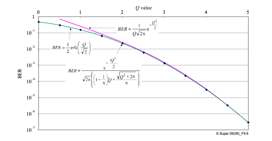
Before we delve into the impact of data rate and modulation, let’s first clarify what BER means and how it is calculated. BER is expressed as a ratio of the number of received bits with errors to the total number of bits transmitted. For example, a BER of 10^-6 means that one out of every million bits transmitted contains an error.

The BER can be calculated using the formula: BER = (Number of bits received with errors) / (Total number of bits transmitted)

The lower the BER, the higher the quality of data transmission, as fewer errors mean better accuracy and reliability. However, achieving a low BER is not an easy task, as various factors can affect it, as we will see in the following sections.

The Role of Data Rate

Data rate refers to the number of bits transmitted per second over an optical link. The higher the data rate, the faster the transmission speed, but also the higher the potential for errors. This is because a higher data rate means that more bits are being transmitted within a given time frame, and this increases the likelihood of errors due to noise, distortion, or other interferences.

As a result, higher data rates generally lead to a higher BER. However, this is not always the case, as other factors such as modulation can also affect the BER, as we will discuss in the following section.

The Role of Modulation

Modulation refers to the technique of encoding data onto an optical carrier signal, which is then transmitted over an optical link. Modulation allows multiple bits to be transmitted within a single symbol, which can increase the data rate and improve the spectral efficiency of optical links.

However, different modulation schemes have different levels of sensitivity to noise and other interferences, which can affect the BER. For example, amplitude modulation (AM) and frequency modulation (FM) are more susceptible to noise, while phase modulation (PM) and quadrature amplitude modulation (QAM) are more robust against noise.

Therefore, the choice of modulation scheme can significantly impact the BER, as some schemes may perform better than others at a given data rate.

BER vs. Data Rate

As we have seen, data rate and modulation can both affect the BER of optical links. However, the question remains: which factor has a more significant impact on BER? The answer is not straightforward, as both factors interact in complex ways and depend on the specific design and configuration of the optical link.

Generally speaking, higher data rates tend to lead to higher BER, as more bits are transmitted per second, increasing the likelihood of errors. However, this relationship is not linear, as other factors such as the quality of the transmitter and receiver, the signal-to-noise ratio, and the modulation scheme can all influence the BER. In some cases, increasing the data rate can improve the BER by allowing the use of more robust modulation schemes or improving the receiver’s sensitivity.

Moreover, different types of data may have different BER requirements, depending on their importance and the desired level of accuracy. For example, video data may be more tolerant of errors than financial data, which requires high accuracy and reliability.

BER vs. Modulation

Modulation is another critical factor that affects the BER of optical links. As we mentioned earlier, different modulation schemes have different levels of sensitivity to noise and other interferences, which can impact the BER. For example, QAM can achieve higher data rates than AM or FM, but it is also more susceptible to noise and distortion.

Therefore, the choice of modulation scheme should take into account the desired data rate, the noise level, and the quality of the transmitter and receiver. In some cases, a higher data rate may not be achievable or necessary, and a more robust modulation scheme may be preferred to improve the BER.

Real-World Examples

To illustrate the impact of data rate and modulation on BER, let’s consider two real-world examples.

In the first example, a telecom company wants to transmit high-quality video data over a long-distance optical link. The desired data rate is 1 Gbps, and the BER requirement is 10^-9. The company can choose between two modulation schemes: QAM and amplitude-shift keying (ASK).

QAM can achieve a higher data rate of 1 Gbps, but it is also more sensitive to noise and distortion, which can increase the BER. ASK, on the other hand, has a lower data rate of 500 Mbps but is more robust against noise and can achieve a lower BER. Therefore, depending on the noise level and the quality of the transmitter and receiver, the telecom company may choose ASK over QAM to meet its BER requirement.

In the second example, a financial institution wants to transmit sensitive financial data over a short-distance optical link. The desired data rate is 10 Mbps, and the BER requirement is 10^-12. The institution can choose between two data rates: 10 Mbps and 100 Mbps, both using PM modulation.

Although the higher data rate of 100 Mbps can achieve faster transmission, it may not be necessary for financial data, which requires high accuracy and reliability. Therefore, the institution may choose the lower data rate of 10 Mbps, which can achieve a lower BER and meet its accuracy requirements.

Conclusion

In conclusion, BER is a crucial metric in optical communication, and its value heavily depends on various factors, including data rate and modulation. Higher data rates tend to lead to higher BER, but other factors such as modulation schemes, noise level, and the quality of the transmitter and receiver can also influence the BER. Therefore, the choice of data rate and modulation should take into account the specific design and requirements of the optical link, as well as the type and importance of the transmitted data.

FAQs

What is BER in optical communication?

BER stands for Bit Error Rate, which measures the probability of errors in digital data transmission over optical links.

What factors affect the BER in optical communication?

Various factors can affect the BER in optical communication, including data rate, modulation, the quality of the transmitter and receiver, the signal-to-noise ratio, and the type and importance of the transmitted data.

Does a higher data rate always lead to a higher BER in optical communication?

Not necessarily. Although higher data rates generally lead to a higher BER, other factors such as modulation schemes, noise level, and the quality of the transmitter and receiver can also influence the BER.

What is the role of modulation in optical communication?

Modulation allows data to be encoded onto an optical carrier signal, which is then transmitted over an optical link. Different modulation schemes have different levels of sensitivity to noise and other interferences, which can impact the BER.

How do real-world examples illustrate the impact of data rate and modulation on BER?

Real-world examples can demonstrate the interaction and trade-offs between data rate and modulation in achieving the desired BER and accuracy requirements for different types of data and applications. By considering specific scenarios and constraints, we can make informed decisions about the optimal data rate and modulation scheme for a given optical link.

In Technical 6 Mins Read

Does OSNR Depend on Data Rate or Modulation in DWDM Link?

In this article, we explore whether OSNR (Optical Signal-to-Noise Ratio) depends on data rate or modulation in DWDM (Dense Wavelength Division Multiplexing) link. We delve into the technicalities and provide a comprehensive overview of this important topic.

Introduction

OSNR is a crucial parameter in optical communication systems that determines the quality of the optical signal. It measures the ratio of the signal power to the noise power in a given bandwidth. The higher the OSNR value, the better the signal quality and the more reliable the communication link.

DWDM technology is widely used in optical communication systems to increase the capacity of fiber optic networks. It allows multiple optical signals to be transmitted over a single fiber by using different wavelengths of light. However, as the number of wavelengths and data rates increase, the OSNR value may decrease, which can lead to signal degradation and errors.

In this article, we aim to answer the question of whether OSNR depends on data rate or modulation in DWDM link. We will explore the technical aspects of this topic and provide a comprehensive overview to help readers understand this important parameter.

Does OSNR Depend on Data Rate?

The data rate is the amount of data that can be transmitted per unit time, usually measured in bits per second (bps). In DWDM systems, the data rate can vary depending on the modulation scheme and the number of wavelengths used. The higher the data rate, the more information can be transmitted over the network.

One might assume that the OSNR value would decrease as the data rate increases. This is because a higher data rate requires a larger bandwidth, which means more noise is present in the signal. However, this assumption is not entirely correct.

In fact, the OSNR value depends on the signal bandwidth, not the data rate. The bandwidth of the signal is determined by the modulation scheme used. For example, a higher-order modulation scheme, such as QPSK (Quadrature Phase-Shift Keying), has a narrower bandwidth than a lower-order modulation scheme, such as BPSK (Binary Phase-Shift Keying).

Therefore, the OSNR value is not directly dependent on the data rate, but rather on the modulation scheme used to transmit the data. In other words, a higher data rate can be achieved with a narrower bandwidth by using a higher-order modulation scheme, which can maintain a high OSNR value.

Does OSNR Depend on Modulation?

As mentioned earlier, the OSNR value depends on the signal bandwidth, which is determined by the modulation scheme used. Therefore, the OSNR value is directly dependent on the modulation scheme used in the DWDM system.

The modulation scheme determines how the data is encoded onto the optical signal. There are several modulation schemes used in optical communication systems, including BPSK, QPSK, 8PSK (8-Phase-Shift Keying), and 16QAM (16-Quadrature Amplitude Modulation).

In general, higher-order modulation schemes have a higher data rate but a narrower bandwidth, which means they can maintain a higher OSNR value. However, higher-order modulation schemes are also more susceptible to noise and other impairments in the communication link.

Therefore, the choice of modulation scheme depends on the specific requirements of the communication system. If a high data rate is required, a higher-order modulation scheme can be used, but the OSNR value may decrease. On the other hand, if a high OSNR value is required, a lower-order modulation scheme can be used, but the data rate may be lower.

Pros and Cons of Different Modulation Schemes

Different modulation schemes have their own advantages and disadvantages, which must be considered when choosing a scheme for a particular communication system.

BPSK (Binary Phase-Shift Keying)

BPSK is a simple modulation scheme that encodes data onto a carrier wave by shifting the phase of the wave by 180 degrees for a “1” bit and leaving it unchanged for a “0” bit. BPSK has a relatively low data rate but is less susceptible to noise and other impairments in the communication link.

Pros:

Simple modulation scheme
Low susceptibility to noise

Cons:

Low data rate
Narrow bandwidth

QPSK (Quadrature Phase-Shift Keying)

QPSK is a more complex modulation scheme that encodes data onto a carrier wave by shifting the phase of the wave by 90, 180, 270, or 0 degrees for each symbol. QPSK has a higher data rate than BPSK but is more susceptible to noise and other impairments in the communication link.

Pros:

Higher data rate than BPSK
More efficient use of bandwidth

Cons:

More susceptible to noise than BPSK

8PSK (8-Phase-Shift Keying)

8PSK is a higher-order modulation scheme that encodes data onto a carrier wave by shifting the phase of the wave by 45, 90, 135, 180, 225, 270, 315, or 0 degrees for each symbol. 8PSK has a higher data rate than QPSK but is more susceptible to noise and other impairments in the communication link.

Pros:

Higher data rate than QPSK
More efficient use of bandwidth

Cons:

More susceptible to noise than QPSK

16QAM (16-Quadrature Amplitude Modulation)

16QAM is a high-order modulation scheme that encodes data onto a carrier wave by modulating the amplitude and phase of the wave. 16QAM has a higher data rate than 8PSK but is more susceptible to noise and other impairments in the communication link.

Pros:

Highest data rate of all modulation schemes
More efficient use of bandwidth

Cons:

Most susceptible to noise and other impairments

Conclusion

In conclusion, the OSNR value in a DWDM link depends on the modulation scheme used and the signal bandwidth, rather than the data rate. Higher-order modulation schemes have a higher data rate but a narrower bandwidth, which can result in a lower OSNR value. Lower-order modulation schemes have a wider bandwidth, which can result in a higher OSNR value but a lower data rate.

Ultimately, the selection of the appropriate modulation scheme and other parameters in a DWDM link requires careful consideration of the specific application and requirements of the communication system.

In Technical 3 Mins Read

Understanding Noise Figure in Amplifiers: Definition, Importance, and How to Reduce It

When working with amplifiers, grasping the concept of noise figure is essential. This article aims to elucidate noise figure, its significance, methods for its measurement and reduction in amplifier designs. Additionally, we’ll provide the correct formula for calculating noise figure and an illustrative example.

What is Noise Figure in Amplifiers?
Why is Noise Figure Important in Amplifiers?
How to Measure Noise Figure in Amplifiers
Factors Affecting Noise Figure in Amplifiers
How to Reduce Noise Figure in Amplifier Design
Formula for Calculating Noise Figure
Example of Calculating Noise Figure
Conclusion
FAQs

What is Noise Figure in Amplifiers?

Noise figure quantifies the additional noise an amplifier introduces to a signal, expressed as the ratio between the signal-to-noise ratio (SNR) at the amplifier’s input and output, both measured in decibels (dB). It’s a pivotal parameter in amplifier design and selection.

Why is Noise Figure Important in Amplifiers?

In applications where SNR is critical, such as communication systems, maintaining a low noise figure is paramount to prevent signal degradation over long distances. Optimizing the noise figure in amplifier design enhances amplifier performance for specific applications.

How to Measure Noise Figure in Amplifiers

Noise figure measurement requires specialized tools like a noise figure meter, which outputs a known noise signal to measure the SNR at both the amplifier’s input and output. This allows for accurate determination of the noise added by the amplifier.

Factors Affecting Noise Figure in Amplifiers

Various factors influence amplifier noise figure, including the amplifier type, operation frequency (higher frequencies typically increase noise figure), and operating temperature (with higher temperatures usually raising the noise figure).

How to Reduce Noise Figure in Amplifier Design

Reducing noise figure can be achieved by incorporating a low-noise amplifier (LNA) at the input stage, applying negative feedback (which may lower gain), employing a balanced or differential amplifier, and minimizing amplifier temperature.

Formula for Calculating Noise Figure

The correct formula for calculating the noise figure is:

NF(dB) = SNRin (dB) −SNRout (dB)

Where NF is the noise figure in dB, SNR_in is the input signal-to-noise ratio, and SNR_out is the output signal-to-noise ratio.

Example of Calculating Noise Figure

Consider an amplifier with an input SNR of 20 dB and an output SNR of 15 dB. The noise figure is calculated as:

NF= 20 dB−15 dB =5dB

Thus, the amplifier’s noise figure is 5 dB.

Conclusion

Noise figure is an indispensable factor in amplifier design, affecting signal quality and performance. By understanding and managing noise figure, amplifiers can be optimized for specific applications, ensuring minimal signal degradation over distances. Employing strategies like using LNAs and negative feedback can effectively minimize noise figure.

FAQs

What’s the difference between noise figure and noise temperature?
- Noise figure measures the noise added by an amplifier, while noise temperature represents the noise’s equivalent temperature.
Why is a low noise figure important in communication systems?
- A low noise figure ensures minimal signal degradation over long distances in communication systems.
How is noise figure measured?
- Noise figure is measured using a noise figure meter, which assesses the SNR at the amplifier’s input and output.
Can noise figure be negative?
- No, the noise figure is always greater than or equal to 0 dB.
How can I reduce the noise figure in my amplifier design?
- Reducing the noise figure can involve using a low-noise amplifier, implementing negative feedback, employing a balanced or differential amplifier, and minimizing the amplifier’s operating temperature.

In Technical 2 Mins Read

Relationship between Q Factor and Data Rate or Modulation: Analysis and Examples

As the data rate and complexity of the modulation format increase, the system becomes more sensitive to noise, dispersion, and nonlinear effects, resulting in a higher required Q factor to maintain an acceptable BER.

The Q factor (also called Q-factor or Q-value) is a dimensionless parameter that represents the quality of a signal in a communication system, often used to estimate the Bit Error Rate (BER) and evaluate the system’s performance. The Q factor is influenced by factors such as noise, signal-to-noise ratio (SNR), and impairments in the optical link. While the Q factor itself does not directly depend on the data rate or modulation format, the required Q factor for a specific system performance does depend on these factors.

Let’s consider some examples to illustrate the impact of data rate and modulation format on the Q factor:

Data Rate:

Example 1: Consider a DWDM system using Non-Return-to-Zero (NRZ) modulation format at 10 Gbps. If the system is properly designed and optimized, it may achieve a Q factor of 20.

Example 2: Now consider the same DWDM system using NRZ modulation format, but with a higher data rate of 100 Gbps. The higher data rate makes the system more sensitive to noise and impairments like chromatic dispersion and polarization mode dispersion. As a result, the required Q factor to achieve the same BER might increase (e.g., 25).

Modulation Format:

Example 1: Consider a DWDM system using NRZ modulation format at 10 Gbps. If the system is properly designed and optimized, it may achieve a Q factor of 20.

Example 2: Now consider the same DWDM system using a more complex modulation format, such as 16-QAM (Quadrature Amplitude Modulation), at 10 Gbps. The increased complexity of the modulation format makes the system more sensitive to noise, dispersion, and nonlinear effects. As a result, the required Q factor to achieve the same BER might increase (e.g., 25).

These examples show that the required Q factor to maintain a specific system performance can be affected by the data rate and modulation format. To achieve a high Q factor at higher data rates and more complex modulation formats, it is crucial to optimize the system design, including factors such as dispersion management, nonlinear effects mitigation, and the implementation of Forward Error Correction (FEC) mechanisms.

In Technical 4 Mins Read

Analysis of OSNR and Q Factor Performance for Different Data Rates and Modulation Formats