In Technical 4 Mins Read

Exploring the C+L Bands in DWDM Network

By MapYourTech April 16, 2024

Exploring the C+L Bands in DWDM Network

DWDM networks have traditionally operated within the C-band spectrum due to its lower dispersion and the availability of efficient Erbium-Doped Fiber Amplifiers (EDFAs). Initially, the C-band supported a spectrum of 3.2 terahertz (THz), which has been expanded to 4.8 THz to accommodate increased data traffic. While the Japanese market favored the L-band early on, this preference is now expanding globally as the L-band’s ability to double the spectrum capacity becomes crucial. The integration of the L-band adds another 4.8 THz, resulting in a total of 9.6 THz when combined with the C-band.

What Does C+L Mean?

C+L band refers to two specific ranges of wavelengths used in optical fiber communications: the C-band and the L-band. The C-band ranges from approximately 1530 nm to 1565 nm, while the L-band covers from about 1565 nm to 1625 nm. These bands are crucial for transmitting signals over optical fiber, offering distinct characteristics in terms of attenuation, dispersion, and capacity.

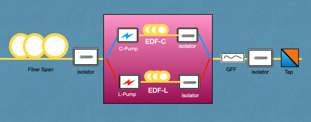
C+L Architecture

The Advantages of C+L

The adoption of C+L bands in fiber optic networks comes with several advantages, crucial for meeting the growing demands for data transmission and communication services:

Increased Capacity: One of the most significant advantages of utilizing both C and L bands is the dramatic increase in network capacity. By essentially doubling the available spectrum for data transmission, service providers can accommodate more data traffic, which is essential in an era where data consumption is soaring due to streaming services, IoT devices, and cloud computing.
Improved Efficiency: The use of C+L bands makes optical networks more efficient. By leveraging wider bandwidths, operators can optimize their existing infrastructure, reducing the need for additional physical fibers. This efficiency not only cuts costs but also accelerates the deployment of new services.
Enhanced Flexibility: With more spectrum comes greater flexibility in managing and allocating resources. Network operators can dynamically adjust bandwidth allocations to meet changing demand patterns, improving overall service quality and user experience.
Reduced Attenuation and Dispersion: Each band has its own set of optical properties. By carefully managing signals across both C and L bands, it’s possible to mitigate issues like signal attenuation and chromatic dispersion, leading to longer transmission distances without the need for signal regeneration.

Challenges in C+L Band Implementation:

Stimulated Raman Scattering (SRS): A significant challenge in C+L band usage is SRS, which causes a tilt in power distribution from the C-band to the L-band. This effect can create operational issues, such as longer recovery times from network failures, slow and complex provisioning due to the need to manage the power tilt between the bands, and restrictions on network topologies.
Cost: The financial aspect is another hurdle. Doubling the components, such as amplifiers and wavelength-selective switches (WSS), can be costly. Network upgrades from C-band to C+L can often mean a complete overhaul of the existing line system, a deterrent for many operators if the L-band isn’t immediately needed.
C+L Recovery Speed: Network recovery from failures can be sluggish, with times hovering around the 10-minute mark.
C+L Provisioning Speed and Complexity: The provisioning process becomes more complicated, demanding careful management of the number of channels across bands.

The Future of C+L

The future of C+L in optical communications is bright, with several trends and developments on the horizon:

Integration with Emerging Technologies: As 5G and beyond continue to roll out, the integration of C+L band capabilities with these new technologies will be crucial. The increased bandwidth and efficiency will support the ultra-high-speed, low-latency requirements of future mobile networks and applications.
Innovations in Fiber Optic Technology: Ongoing research in fiber optics, including new types of fibers and advanced modulation techniques, promises to further unlock the potential of the C+L bands. These innovations could lead to even greater capacities and more efficient use of the optical spectrum.
Sustainability Impacts: With an emphasis on sustainability, the efficiency improvements associated with C+L band usage could contribute to reducing the energy consumption of data centers and network infrastructure, aligning with global efforts to minimize environmental impacts.
Expansion Beyond Telecommunications: While currently most relevant to telecommunications, the benefits of C+L band technology could extend to other areas, including remote sensing, medical imaging, and space communications, where the demand for high-capacity, reliable transmission is growing.

In conclusion, the adoption and development of C+L band technology represent a significant step forward in the evolution of optical communications. By offering increased capacity, efficiency, and flexibility, C+L bands are well-positioned to meet the current and future demands of our data-driven world. As we look to the future, the continued innovation and integration of C+L technology into broader telecommunications and technology ecosystems will be vital in shaping the next generation of global communication networks.

References:

In Technical 3 Mins Read

Linear and Nonlinear Degradations in Fiber Optic Systems

By MapYourTech April 1, 2024

In the world of fiber-optic communication, the integrity of the transmitted signal is critical. As an optical engineers, our primary objective is to mitigate the attenuation of signals across long distances, ensuring that data arrives at its destination with minimal loss and distortion. In this article we will discuss into the challenges of linear and nonlinear degradations in fiber-optic systems, with a focus on transoceanic length systems, and offers strategies for optimising system performance.

The Role of Optical Amplifiers

Erbium-doped fiber amplifiers (EDFAs) are the cornerstone of long-distance fiber-optic transmission, providing essential gain within the low-loss window around 1550 nm. Positioned typically between 50 to 100 km apart, these amplifiers are critical for compensating the fiber’s inherent attenuation. Despite their crucial role, EDFAs introduce additional noise, progressively degrading the optical signal-to-noise ratio (OSNR) along the transmission line. This degradation necessitates a careful balance between signal amplification and noise management to maintain transmission quality.

OSNR: The Critical Metric

The received OSNR, a key metric for assessing channel performance, is influenced by several factors, including the channel’s fiber launch power, span loss, and the noise figure (NF) of the EDFA. The relationship is outlined as follows:

Where:

$N EDFA$ is the number of EDFAs the signal has passed through.
$P Launch$ is the power of the signal when it’s first sent into the fiber, in dBm.
Loss represents the total loss the signal experiences, in dB.
NF is the noise figure of the EDFA, also in dB.

Increasing the launch power enhances the OSNR linearly; however, this is constrained by the onset of fiber nonlinearity, particularly Kerr effects, which limit the maximum effective launch power.

The Kerr Effect and Its Implications

The Kerr effect, stemming from the intensity-dependent refractive index of optical fiber, leads to modulation in the fiber’s refractive index and subsequent optical phase changes. Despite the Kerr coefficient ( $n_{2}$ ) being exceedingly small, the combined effect of long transmission distances, high total power from EDFAs, and the small effective area of standard single-mode fiber (SMF) renders this nonlinearity a dominant factor in signal degradation over transoceanic distances.

The phase change induced by this effect depends on a few key factors:

The fiber’s nonlinear coefficient $n_{2}$ .
The signal power $P_{s} (t)$ , which varies over time.
The transmission distance.
The fiber’s effective area $A eff$ .

This phase modulation complicates the accurate recovery of the transmitted optical field, thus limiting the achievable performance of undersea fiber-optic transmission systems.

The Kerr effect is a bit like trying to talk to someone at a party where the music volume keeps changing. Sometimes your message gets through loud and clear, and other times it’s garbled by the fluctuations. In fiber optics, managing these fluctuations is crucial for maintaining signal integrity over long distances.

Striking the Right Balance

Understanding and mitigating the effects of both linear and nonlinear degradations are critical for optimising the performance of undersea fiber-optic transmission systems. Engineers must navigate the delicate balance between maximizing OSNR for enhanced signal quality and minimising the impact of nonlinear distortions.The trick, then, is to find that sweet spot where our OSNR is high enough to ensure quality transmission but not so high that we’re deep into the realm of diminishing returns due to nonlinear degradation. Strategies such as carefully managing launch power, employing advanced modulation formats, and leveraging digital signal processing techniques are vital for overcoming these challenges.

In Technical 3 Mins Read

ZR vs. ZR+: Navigating the Evolution of Coherent Optical Standards

By MapYourTech March 30, 2024

In this ever-evolving landscape of optical networking, the development of coherent optical standards, such as 400G ZR and ZR+, represents a significant leap forward in addressing the insatiable demand for bandwidth, efficiency, and scalability in data centers and network infrastructure. This technical blog delves into the nuances of these standards, comparing their features, applications, and how they are shaping the future of high-capacity networking.

Introduction to 400G ZR

The 400G ZR standard, defined by the Optical Internetworking Forum (OIF), is a pivotal development in the realm of optical networking, setting the stage for the next generation of data transmission over optical fiber’s. It is designed to facilitate the transfer of 400 Gigabit Ethernet over single-mode fiber across distances of up to 120 kilometers without the need for signal amplification or regeneration. This is achieved through the use of advanced modulation techniques like DP-16QAM and state-of-the-art forward error correction (FEC).

Key features of 400G ZR include:

High Capacity: Supports the transmission of 400 Gbps using a single wavelength.
Compact Form-Factor: Integrates into QSFP-DD and OSFP modules, aligning with industry standards for data center equipment.
Cost Efficiency: Reduces the need for external transponders and simplifies network architecture, lowering both CAPEX and OPEX.

Emergence of 400G ZR+

Building upon the foundation set by 400G ZR, the 400G ZR+ standard extends the capabilities of its predecessor by increasing the transmission reach and introducing flexibility in modulation schemes to cater to a broader range of network topologies and distances. The OpenZR+ MSA has been instrumental in this expansion, promoting interoperability and open standards in coherent optics.

Key enhancements in 400G ZR+ include:

Extended Reach: With advanced FEC and modulation, ZR+ can support links up to 2,000 km, making it suitable for longer metro, regional, and even long-haul deployments.
Versatile Modulation: Offers multiple configuration options (e.g., DP-16QAM, DP-8QAM, DP-QPSK), enabling operators to balance speed, reach, and optical performance.
Improved Power Efficiency: Despite its extended capabilities, ZR+ maintains a focus on energy efficiency, crucial for reducing the environmental impact of expanding network infrastructures.

ZR vs. ZR+: A Comparative Analysis

Feature.	400G ZR	400G ZR+
Reach	Up to 120 km	Up to 2,000 km
Modulation	DP-16QAM	DP-16QAM, DP-8QAM, DP-QPSK
Form Factor	QSFP-DD, OSFP	QSFP-DD, OSFP
Application	Data center interconnects	Metro, regional, long-haul

Adding few more interesting table for readers

The Future Outlook

The advent of 400G ZR and ZR+ is not just a technical upgrade; it’s a paradigm shift in how we approach optical networking. With these technologies, network operators can now deploy more flexible, efficient, and scalable networks, ready to meet the future demands of data transmission.

Moreover, the ongoing development and expected introduction of XR optics highlight the industry’s commitment to pushing the boundaries of what’s possible in optical networking. XR optics, with its promise of multipoint capabilities and aggregation of lower-speed interfaces, signifies the next frontier in coherent optical technology.

In Technical 2 Mins Read

OSNR Calculation for an Amplified Cascaded Span

By MapYourTech January 31, 2024

When we’re dealing with Optical Network Elements (ONEs) that include optical amplifiers, it’s important to note a key change in signal quality. Specifically, the Optical Signal-to-Noise Ratio (OSNR) at the points where the signal exits the system or at drop ports, is typically not as high as the OSNR where the signal enters or is added to the system. This decrease in signal quality is a critical factor to consider, and there’s a specific equation that allows us to quantify this reduction in OSNR. By using following equations, network engineers can effectively calculate and predict the change in OSNR, ensuring that the network’s performance meets the necessary standards.

Where:

osnr_out : linear OSNR at the output port of the ONE

osnr_in : linear OSNR at the input port of the ONE

osnr_one : linear OSNR that would appear at the output port of the ONE for a noise free input signal

If the OSNR is defined in logarithmic terms (dB) and the equation(Eq.1) for the OSNR due to the ONE being considered is substituted this equation becomes:

Where:

OSNR_out : log OSNR (dB) at the output port of the ONE

OSNR_in : log OSNR (dB) at the input port of the ONE

P_in : channel power (dBm) at the input port of the ONE

NF : noise figure (dB) of the relevant path through the ONE

h : Planck’s constant (in mJ•s to be consistent with in P_in (dBm))

v : optical frequency in Hz

v_r : reference bandwidth in Hz (usually the frequency equivalent of 0.1 nm)

So if it needs to generalised the equation of an end to end point to point link, the equation can be written as

Where:

P_in1, P_in2 to P_inN : channel powers (dBm) at the inputs of the amplifiers or ONEs on the relevant path through the network

NF₁, NF₂ to NF_N : noise figures (dB) of the amplifiers or ONEs on the relevant path through the network

The required OSNR_out value that is needed to meet the required system BER depends on many factors such as the bit rate, whether and what type of FEC is employed, the magnitude of any crosstalk or non-linear penalties in the DWDM line segments etc.Furthermore it will be discuss in another article.

Ref:

ITU-T G.680

In Technical 2 Mins Read

Spectral Grids and WDM Techniques for Fiber Optic Capacity

By MapYourTech January 2, 2024

Introduction

The telecommunications industry constantly strives to maximize the use of fiber optic capacity. Despite the broad spectral width of the conventional C-band, which offers over 40 THz, the limited use of optical channels at 10 or 40 Gbit/s results in substantial under utilization. The solution lies in Wavelength Division Multiplexing (WDM), a technique that can significantly increase the capacity of optical fibers.

Understanding Spectral Grids

WDM employs multiple optical carriers, each on a different wavelength, to transmit data simultaneously over a single fiber. This method vastly improves the efficiency of data transmission, as outlined in ITU-T Recommendations that define the spectral grids for WDM applications.

The Evolution of Channel Spacing

Historically, WDM systems have evolved to support an array of channel spacings. Initially, a 100 GHz grid was established, which was then subdivided by factors of two to create a variety of frequency grids, including:

12.5 GHz spacing
25 GHz spacing
50 GHz spacing
100 GHz spacing

All four frequency grids incorporate 193.1 THz and are not limited by frequency boundaries. Additionally, wider spacing grids can be achieved by using multiples of 100 GHz, such as 200 GHz, 300 GHz, and so on.

ITU-T Recommendations for DWDM

ITU-T Recommendations such as ITU-T G.692 and G.698 series outline applications utilizing these DWDM frequency grids. The recent addition of a flexible DWDM grid, as per Recommendation ITU-T G.694.1, allows for variable bit rates and modulation formats, optimizing the allocation of frequency slots to match specific bandwidth requirements.

Flexible DWDM Grid in Practice

The flexible grid is particularly innovative, with nominal central frequencies at intervals of 6.25 GHz from 193.1 THz and slot widths based on 12.5 GHz increments. This flexibility ensures that the grid can adapt to a variety of transmission needs without overlap, as depicted in Figure above.

CWDM Wavelength Grid and Applications

Recommendation ITU-T G.694.2 defines the CWDM wavelength grid to support applications requiring simultaneous transmission of several wavelengths. The 20 nm channel spacing is a result of manufacturing tolerances, temperature variations, and the need for a guardband to use cost-effective filter technologies. These CWDM grids are further detailed in ITU-T G.695.

Conclusion

The strategic use of DWDM and CWDM grids, as defined by ITU-T Recommendations, is key to maximizing the capacity of fiber optic transmissions. With the introduction of flexible grids and ongoing advancements, we are witnessing a transformative period in fiber optic technology.

In Standards 3 Mins Read

ITU-T Recommendations for Optical Fibers and Cables

By MapYourTech January 2, 2024

In the realm of telecommunications, the precision and reliability of optical fibers and cables are paramount. The International Telecommunication Union (ITU) plays a crucial role in this by providing a series of recommendations that serve as global standards. The ITU-T G.650.x and G.65x series of recommendations are especially significant for professionals in the field. In this article, we delve into these recommendations and their interrelationships, as illustrated in Figure 1 .

ITU-T G.650.x Series: Definitions and Test Methods

The ITU-T G.650.x series is foundational for understanding single-mode fibers and cables. ITU-T G.650.1 is the cornerstone, offering definitions and test methods for linear and deterministic parameters of single-mode fibers. This includes key measurements like attenuation and chromatic dispersion, which are critical for ensuring fiber performance over long distances.

Moving forward, ITU-T G.650.2 expands on the initial parameters by providing definitions and test methods for statistical and non-linear parameters. These are essential for predicting fiber behavior under varying signal powers and during different transmission phenomena.

For those involved in assessing installed fiber links, ITU-T G.650.3 offers valuable test methods. It’s tailored to the needs of field technicians and engineers who analyze the performance of installed single-mode fiber cable links, ensuring that they meet the necessary standards for data transmission.

ITU-T G.65x Series: Specifications for Fibers and Cables

The ITU-T G.65x series recommendations provide specifications for different types of optical fibers and cables. ITU-T G.651.1 targets the optical access network with specifications for 50/125 µm multimode fiber and cable, which are widely used in local area networks and data centers due to their ability to support high data rates over short distances.

The series then progresses through various single-mode fiber specifications:

ITU-T G.652: The standard single-mode fiber, suitable for a wide range of applications.
ITU-T G.653: Dispersion-shifted fibers optimized for minimizing chromatic dispersion.
ITU-T G.654: Features a cut-off shifted fiber, often used for submarine cable systems.
ITU-T G.655: Non-zero dispersion-shifted fibers, which are ideal for long-haul transmissions.
ITU-T G.656: Fibers designed for a broader range of wavelengths, expanding the capabilities of dense wavelength division multiplexing systems.
ITU-T G.657: Bending loss insensitive fibers, offering robust performance in tight bends and corners.

Historical Context and Current References

It’s noteworthy to mention that the multimode fiber test methods were initially described in ITU-T G.651. However, this recommendation was deleted in 2008, and now the test methods for multimode fibers are referenced in existing IEC documents. Professionals seeking current standards for multimode fiber testing should refer to these IEC documents for the latest guidelines.

Conclusion

The ITU-T recommendations play a critical role in the standardization and performance optimization of optical fibers and cables. By adhering to these standards, industry professionals can ensure compatibility, efficiency, and reliability in fiber optic networks. Whether you are a network designer, a field technician, or an optical fiber manufacturer, understanding these recommendations is crucial for maintaining the high standards expected in today’s telecommunication landscape.

Reference

https://www.itu.int/rec/T-REC-G/e

In Technical 2 Mins Read

Effects of Channel Spacing on Q Factor in Optical Systems

By MapYourTech December 15, 2023

Channel spacing, the distance between adjacent channels in a WDM system, greatly impacts the overall capacity and efficiency of optical networks. A fundamental rule of thumb is to ensure that the channel spacing is at least four times the bit rate. This principle helps in mitigating interchannel crosstalk, a significant factor that can compromise the integrity of the transmitted signal.

For example, in a WDM system operating at a bit rate of 10 Gbps, the ideal channel spacing should be no less than 40 GHz. This spacing helps in reducing the interference between adjacent channels, thus enhancing the system’s performance.

The Q factor, a measure of the quality of the optical signal, is directly influenced by the chosen channel spacing. It is evaluated at various stages of the transmission, notably at the output of both the multiplexer and the demultiplexer. In a practical scenario, consider a 16-channel DWDM system, where the Q factor is assessed over a transmission distance, taking into account a residual dispersion akin to 10km of Standard Single-Mode Fiber (SSMF). This evaluation is crucial in determining the system’s effectiveness in maintaining signal integrity over long distances.

Studies have shown that when the channel spacing is narrowed to 20–30 GHz, there is a significant drop in the Q factor at the demultiplexer’s output. This reduction indicates a higher level of signal degradation due to closer channel spacing. However, when the spacing is expanded to 40 GHz, the decline in the Q factor is considerably less pronounced. This observation underscores the resilience of certain modulation formats, like the Vestigial Sideband (VSB), against the effects of chromatic dispersion.

In Technical 4 Mins Read

Exploring the Constraints on Fiber Pairs In Submarine Optical Fiber Networks

By MapYourTech August 12, 2023

In the world of global communication, Submarine Optical Fiber Networks cable play a pivotal role in facilitating the exchange of data across continents. As technology continues to evolve, the capacity and capabilities of these cables have been expanding at an astonishing pace. In this article, we delve into the intricate details of how future cables are set to scale their cross-sectional capacity, the factors influencing their design, and the innovative solutions being developed to overcome the challenges posed by increasing demands.

Scaling Factors: WDM Channels, Modes, Cores, and Fibers

In the quest for higher data transfer rates, the architecture of future undersea cables is set to undergo a transformation. The scaling of cross-sectional capacity hinges on several key factors: the number of Wavelength Division Multiplexing (WDM) channels in a mode, the number of modes in a core, the number of cores in a fiber, and the number of fibers in the cable. By optimizing these parameters, cable operators are poised to unlock unprecedented data transmission capabilities.

Current Deployment and Challenges

Presently, undersea cables commonly consist of four to eight fiber pairs. On land, terrestrial cables have ventured into new territory with remarkably high fiber counts, often based on loose tube structures. A remarkable example of this is the deployment of a 1728-fiber cable across Sydney Harbor, Australia. However, the capacity of undersea cables is not solely determined by fiber count; other factors come into play.

Power Constraints and Spatial Limitations

The maximum number of fibers that can be incorporated into an undersea cable is heavily influenced by two critical factors: electrical power availability and physical space constraints. The optical amplifiers, which are essential for boosting signal strength along the cable, require a certain amount of electrical power. This power requirement is dependent on various parameters, including the overall cable length, amplifier spacing, and the number of amplifiers within each repeater. As cable lengths increase, power considerations become increasingly significant.

Efficiency: Improving Amplifiers for Enhanced Utilisation

Optimising the efficiency of optical amplifiers emerges as a strategic solution to mitigate power constraints. By meticulously adjusting design parameters such as narrowing the optical bandwidth, the loss caused by gain flattening filters can be minimised. This reduction in loss subsequently decreases the necessary pump power for signal amplification. This approach not only addresses power limitations but also maximizes the effective utilisation of resources, potentially allowing for an increased number of fiber pairs within a cable.

Multi-Core Fiber: Opening New Horizons

The concept of multi-core fiber introduces a transformative potential for submarine optical networks. By integrating multiple light-guiding cores within a single physical fiber, the capacity for data transmission can be substantially amplified. While progress has been achieved in the fabrication of multi-core fibers, the development of multi-core optical amplifiers remains a challenge. Nevertheless, promising experiments showcasing successful transmissions over extended distances using multi-core fibers with multiple wavelengths hint at the technology’s promising future.

Technological Solutions: Overcoming Space Constraints

As fiber cores increase in number, so does the need for amplifiers within repeater units. This poses a challenge in terms of available physical space. To combat this, researchers are actively exploring two key technological solutions. The first involves optimising the packaging density of optical components, effectively cramming more functionality into the same space. The second avenue involves the use of photonic integrated circuits (PICs), which enable the integration of multiple functions onto a single chip. Despite their potential, PICs do face hurdles in terms of coupling loss and power handling capabilities.

Navigating the Future

The realm of undersea fiber optic cables is undergoing a remarkable evolution, driven by the insatiable demand for data transfer capacity. As we explore the scaling factors of WDM channels, modes, cores, and fibers, it becomes evident that power availability and physical space are crucial constraints. However, ingenious solutions, such as amplifier efficiency improvements and multi-core fiber integration, hold promise for expanding capacity. The development of advanced technologies like photonic integrated circuits underscores the relentless pursuit of higher data transmission capabilities. As we navigate the intricate landscape of undersea cable design, it’s clear that the future of global communication is poised to be faster, more efficient, and more interconnected than ever before.

Reference and Credits

https://www.sciencedirect.com/book/9780128042694/undersea-fiber-communication-systems

http://submarinecablemap.com/

https://www.telegeography.com

https://infoworldmaps.com/3d-submarine-cable-map/

https://gfycat.com/aptmediocreblackpanther

In Technical 3 Mins Read

Choosing The Right Networking Redundancy: A Close Look At 1+1 Vs. 1:1 Configurations

By MapYourTech April 18, 2023

Introduction

Network redundancy is crucial for ensuring continuous network availability and preventing downtime. Redundancy techniques create backup paths for network traffic in case of failures. In this article, we will compare 1+1 and 1:1 redundancy techniques used in networking to determine which one best suits your networking needs.

1+1 Redundancy Technique

1+1 is a redundancy technique that involves two identical devices: a primary device and a backup device. The primary device handles network traffic normally, while the backup device remains idle. In the event of a primary device failure, the backup device takes over to ensure uninterrupted network traffic. This technique is commonly used in situations where network downtime is unacceptable, such as in telecommunications or financial institutions.

Advantages of 1+1 Redundancy Technique

• High availability: 1+1 redundancy ensures network traffic continues even if one device fails. • Fast failover: Backup device takes over quickly, minimizing network downtime. • Simple implementation: Easy to implement with only two identical devices. • Cost: Can be expensive due to the need for two identical devices.

Disadvantages of 1+1 Redundancy Technique

• Resource utilization: One device remains idle in normal conditions, resulting in underutilization.

1:1 Redundancy Technique

1:1 redundancy involves two identical active devices handling network traffic simultaneously. A failover link seamlessly redirects network traffic to the other device in case of failure. This technique is often used in scenarios where network downtime must be avoided, such as in data centers.

Advantages of 1:1 Redundancy Technique

• High availability: 1:1 redundancy ensures network traffic continues even if one device fails. • Load balancing: Both devices are active simultaneously, optimizing resource utilization. • Fast failover: The other device quickly takes over, minimizing network downtime.

Disadvantages of 1:1 Redundancy Technique

• Cost: Requires two identical devices, which can be costly. • Complex implementation: More intricate than 1+1 redundancy, due to failover link configuration.

Choosing the Right Redundancy Technique

Selecting between 1+1 and 1:1 redundancy techniques depends on your networking needs. Both provide high availability and fast failover, but they differ in cost and complexity.

If cost isn’t a significant concern and maximum availability is required, 1:1 redundancy may be the best choice. Both devices are active, ensuring load balancing and optimal network performance, while fast failover minimizes downtime.

However, if cost matters and high availability is still crucial, 1+1 redundancy may be preferable. With only two identical devices, it is more cost-effective. Any underutilization can be offset by using the idle device for other purposes.

Conclusion

In conclusion, both 1+1 and 1:1 redundancy techniques effectively ensure network availability. By considering the advantages and disadvantages of each technique, you can make an informed decision on the best option for your networking needs.

In Interviews 5 Mins Read

OSNR & Q-factor Dependency: Understanding The Impact On Signal Quality And Network Performance

By MapYourTech April 16, 2023

As communication networks become increasingly dependent on fiber-optic technology, it is essential to understand the quality of the signal in optical links. The two primary parameters used to evaluate the signal quality are Optical Signal-to-Noise Ratio (OSNR) and Q-factor. In this article, we will explore what OSNR and Q-factor are and how they are interdependent with examples for optical link.

Introduction
What is OSNR?
- Definition and Calculation of OSNR
What is Q-factor?
- Definition and Calculation of Q-factor
OSNR and Q-factor Relationship
Examples of OSNR and Q-factor Interdependency
- Example 1: OSNR and Q-factor for Single Wavelength System
- Example 2: OSNR and Q-factor for Multi-Wavelength System
Conclusion
FAQs

1. Introduction

Fiber-optic technology is the backbone of modern communication systems, providing fast, secure, and reliable transmission of data over long distances. However, the signal quality of an optical link is subject to various impairments, such as attenuation, dispersion, and noise. To evaluate the signal quality, two primary parameters are used – OSNR and Q-factor.

In this article, we will discuss what OSNR and Q-factor are, how they are calculated, and their interdependency in optical links. We will also provide examples to help you understand how the OSNR and Q-factor affect optical links.

2. What is OSNR?

OSNR stands for Optical Signal-to-Noise Ratio. It is a measure of the signal quality of an optical link, indicating how much the signal power exceeds the noise power. The higher the OSNR value, the better the signal quality of the optical link.

Definition and Calculation of OSNR

The OSNR is calculated as the ratio of the optical signal power to the noise power within a specific bandwidth. The formula for calculating OSNR is as follows:

OSNR (dB) = 10 log10 (Signal Power / Noise Power)

3. What is Q-factor?

Q-factor is a measure of the quality of a digital signal in an optical communication system. It is a function of the bit error rate (BER), signal power, and noise power. The higher the Q-factor value, the better the quality of the signal.

Definition and Calculation of Q-factor

The Q-factor is calculated as the ratio of the distance between the average signal levels of two adjacent symbols to the standard deviation of the noise. The formula for calculating Q-factor is as follows:

Q-factor = (Signal Level 1 – Signal Level 2) / Noise RMS

4. OSNR and Q-factor Relationship

OSNR and Q-factor are interdependent parameters, meaning that changes in one parameter affect the other. The relationship between OSNR and Q-factor is a logarithmic one, which means that a small change in the OSNR can lead to a significant change in the Q-factor.

Generally, the Q-factor increases as the OSNR increases, indicating a better signal quality. However, at high OSNR values, the Q-factor reaches a saturation point, and further increase in the OSNR does not improve the Q-factor.

5. Examples of OSNR and Q-factor Interdependency

Example 1: OSNR and Q-factor for Single Wavelength System

In a single wavelength system, the OSNR and Q-factor have a direct relationship. An increase in the OSNR improves the Q-factor, resulting in a better signal quality. For instance, if the OSNR of a single wavelength system increases from 20 dB to 30 dB,

the Q-factor also increases, resulting in a lower BER and better signal quality. Conversely, a decrease in the OSNR degrades the Q-factor, leading to a higher BER and poor signal quality.

Example 2: OSNR and Q-factor for Multi-Wavelength System

In a multi-wavelength system, the interdependence of OSNR and Q-factor is more complex. The OSNR and Q-factor of each wavelength in the system can vary independently, and the overall system performance depends on the worst-performing wavelength.

For example, consider a four-wavelength system, where each wavelength has an OSNR of 20 dB, 25 dB, 30 dB, and 35 dB. The Q-factor of each wavelength will be different due to the different noise levels. The overall system performance will depend on the wavelength with the worst Q-factor. In this case, if the Q-factor of the first wavelength is the worst, the system performance will be limited by the Q-factor of that wavelength, regardless of the OSNR values of the other wavelengths.

6. Conclusion

In conclusion, OSNR and Q-factor are essential parameters used to evaluate the signal quality of an optical link. They are interdependent, and changes in one parameter affect the other. Generally, an increase in the OSNR improves the Q-factor and signal quality, while a decrease in the OSNR degrades the Q-factor and signal quality. However, the relationship between OSNR and Q-factor is more complex in multi-wavelength systems, and the overall system performance depends on the worst-performing wavelength.

Understanding the interdependence of OSNR and Q-factor is crucial in designing and optimizing optical communication systems for better performance.

7. FAQs

What is the difference between OSNR and SNR? OSNR is the ratio of signal power to noise power within a specific bandwidth, while SNR is the ratio of signal power to noise power over the entire frequency range.
What is the acceptable range of OSNR and Q-factor in optical communication systems? The acceptable range of OSNR and Q-factor varies depending on the specific application and system design. However, a higher OSNR and Q-factor generally indicate better signal quality.
How can I improve the OSNR and Q-factor of an optical link? You can improve the OSNR and Q-factor of an optical link by reducing noise sources, optimizing system design, and using higher-quality components.
Can I measure the OSNR and Q-factor of an optical link in real-time? Yes, you can measure the OSNR and Q-factor of an optical link in real-time using specialized instruments such as an optical spectrum analyzer and a bit error rate tester.
What are the future trends in optical communication systems regarding OSNR and Q-factor? Future trends in optical communication systems include the development of advanced modulation techniques and the use of machine learning algorithms to optimize system performance and improve the OSNR and Q-factor of optical links.

In Technical 8 Mins Read

Does BER Depend on Data Rate or Modulation?

By MapYourTech April 16, 2023

In the world of optical communication, it is crucial to have a clear understanding of Bit Error Rate (BER). This metric measures the probability of errors in digital data transmission, and it plays a significant role in the design and performance of optical links. However, there are ongoing debates about whether BER depends more on data rate or modulation. In this article, we will explore the impact of data rate and modulation on BER in optical links, and we will provide real-world examples to illustrate our points.

Introduction
Understanding BER
The Role of Data Rate
The Role of Modulation
BER vs. Data Rate
BER vs. Modulation
Real-World Examples
Conclusion
FAQs

Introduction

Optical links have become increasingly essential in modern communication systems, thanks to their high-speed transmission, long-distance coverage, and immunity to electromagnetic interference. However, the quality of optical links heavily depends on the BER, which measures the number of errors in the transmitted bits relative to the total number of bits. In other words, the BER reflects the accuracy and reliability of data transmission over optical links.

BER depends on various factors, such as the quality of the transmitter and receiver, the noise level, and the optical power. However, two primary factors that significantly affect BER are data rate and modulation. There have been ongoing debates about whether BER depends more on data rate or modulation, and in this article, we will examine both factors and their impact on BER.

Understanding BER

Before we delve into the impact of data rate and modulation, let’s first clarify what BER means and how it is calculated. BER is expressed as a ratio of the number of received bits with errors to the total number of bits transmitted. For example, a BER of 10^-6 means that one out of every million bits transmitted contains an error.

The BER can be calculated using the formula: BER = (Number of bits received with errors) / (Total number of bits transmitted)

The lower the BER, the higher the quality of data transmission, as fewer errors mean better accuracy and reliability. However, achieving a low BER is not an easy task, as various factors can affect it, as we will see in the following sections.

The Role of Data Rate

Data rate refers to the number of bits transmitted per second over an optical link. The higher the data rate, the faster the transmission speed, but also the higher the potential for errors. This is because a higher data rate means that more bits are being transmitted within a given time frame, and this increases the likelihood of errors due to noise, distortion, or other interferences.

As a result, higher data rates generally lead to a higher BER. However, this is not always the case, as other factors such as modulation can also affect the BER, as we will discuss in the following section.

The Role of Modulation

Modulation refers to the technique of encoding data onto an optical carrier signal, which is then transmitted over an optical link. Modulation allows multiple bits to be transmitted within a single symbol, which can increase the data rate and improve the spectral efficiency of optical links.

However, different modulation schemes have different levels of sensitivity to noise and other interferences, which can affect the BER. For example, amplitude modulation (AM) and frequency modulation (FM) are more susceptible to noise, while phase modulation (PM) and quadrature amplitude modulation (QAM) are more robust against noise.

Therefore, the choice of modulation scheme can significantly impact the BER, as some schemes may perform better than others at a given data rate.

BER vs. Data Rate

As we have seen, data rate and modulation can both affect the BER of optical links. However, the question remains: which factor has a more significant impact on BER? The answer is not straightforward, as both factors interact in complex ways and depend on the specific design and configuration of the optical link.

Generally speaking, higher data rates tend to lead to higher BER, as more bits are transmitted per second, increasing the likelihood of errors. However, this relationship is not linear, as other factors such as the quality of the transmitter and receiver, the signal-to-noise ratio, and the modulation scheme can all influence the BER. In some cases, increasing the data rate can improve the BER by allowing the use of more robust modulation schemes or improving the receiver’s sensitivity.

Moreover, different types of data may have different BER requirements, depending on their importance and the desired level of accuracy. For example, video data may be more tolerant of errors than financial data, which requires high accuracy and reliability.

BER vs. Modulation

Modulation is another critical factor that affects the BER of optical links. As we mentioned earlier, different modulation schemes have different levels of sensitivity to noise and other interferences, which can impact the BER. For example, QAM can achieve higher data rates than AM or FM, but it is also more susceptible to noise and distortion.

Therefore, the choice of modulation scheme should take into account the desired data rate, the noise level, and the quality of the transmitter and receiver. In some cases, a higher data rate may not be achievable or necessary, and a more robust modulation scheme may be preferred to improve the BER.

Real-World Examples

To illustrate the impact of data rate and modulation on BER, let’s consider two real-world examples.

In the first example, a telecom company wants to transmit high-quality video data over a long-distance optical link. The desired data rate is 1 Gbps, and the BER requirement is 10^-9. The company can choose between two modulation schemes: QAM and amplitude-shift keying (ASK).

QAM can achieve a higher data rate of 1 Gbps, but it is also more sensitive to noise and distortion, which can increase the BER. ASK, on the other hand, has a lower data rate of 500 Mbps but is more robust against noise and can achieve a lower BER. Therefore, depending on the noise level and the quality of the transmitter and receiver, the telecom company may choose ASK over QAM to meet its BER requirement.

In the second example, a financial institution wants to transmit sensitive financial data over a short-distance optical link. The desired data rate is 10 Mbps, and the BER requirement is 10^-12. The institution can choose between two data rates: 10 Mbps and 100 Mbps, both using PM modulation.

Although the higher data rate of 100 Mbps can achieve faster transmission, it may not be necessary for financial data, which requires high accuracy and reliability. Therefore, the institution may choose the lower data rate of 10 Mbps, which can achieve a lower BER and meet its accuracy requirements.

Conclusion

In conclusion, BER is a crucial metric in optical communication, and its value heavily depends on various factors, including data rate and modulation. Higher data rates tend to lead to higher BER, but other factors such as modulation schemes, noise level, and the quality of the transmitter and receiver can also influence the BER. Therefore, the choice of data rate and modulation should take into account the specific design and requirements of the optical link, as well as the type and importance of the transmitted data.

FAQs

What is BER in optical communication?

BER stands for Bit Error Rate, which measures the probability of errors in digital data transmission over optical links.

What factors affect the BER in optical communication?

Various factors can affect the BER in optical communication, including data rate, modulation, the quality of the transmitter and receiver, the signal-to-noise ratio, and the type and importance of the transmitted data.

Does a higher data rate always lead to a higher BER in optical communication?

Not necessarily. Although higher data rates generally lead to a higher BER, other factors such as modulation schemes, noise level, and the quality of the transmitter and receiver can also influence the BER.

What is the role of modulation in optical communication?

Modulation allows data to be encoded onto an optical carrier signal, which is then transmitted over an optical link. Different modulation schemes have different levels of sensitivity to noise and other interferences, which can impact the BER.

How do real-world examples illustrate the impact of data rate and modulation on BER?

Real-world examples can demonstrate the interaction and trade-offs between data rate and modulation in achieving the desired BER and accuracy requirements for different types of data and applications. By considering specific scenarios and constraints, we can make informed decisions about the optimal data rate and modulation scheme for a given optical link.

In Technical 6 Mins Read

Does OSNR Depend on Data Rate or Modulation in DWDM Link?

By MapYourTech April 16, 2023

In this article, we explore whether OSNR (Optical Signal-to-Noise Ratio) depends on data rate or modulation in DWDM (Dense Wavelength Division Multiplexing) link. We delve into the technicalities and provide a comprehensive overview of this important topic.

Introduction

OSNR is a crucial parameter in optical communication systems that determines the quality of the optical signal. It measures the ratio of the signal power to the noise power in a given bandwidth. The higher the OSNR value, the better the signal quality and the more reliable the communication link.

DWDM technology is widely used in optical communication systems to increase the capacity of fiber optic networks. It allows multiple optical signals to be transmitted over a single fiber by using different wavelengths of light. However, as the number of wavelengths and data rates increase, the OSNR value may decrease, which can lead to signal degradation and errors.

In this article, we aim to answer the question of whether OSNR depends on data rate or modulation in DWDM link. We will explore the technical aspects of this topic and provide a comprehensive overview to help readers understand this important parameter.

Does OSNR Depend on Data Rate?

The data rate is the amount of data that can be transmitted per unit time, usually measured in bits per second (bps). In DWDM systems, the data rate can vary depending on the modulation scheme and the number of wavelengths used. The higher the data rate, the more information can be transmitted over the network.

One might assume that the OSNR value would decrease as the data rate increases. This is because a higher data rate requires a larger bandwidth, which means more noise is present in the signal. However, this assumption is not entirely correct.

In fact, the OSNR value depends on the signal bandwidth, not the data rate. The bandwidth of the signal is determined by the modulation scheme used. For example, a higher-order modulation scheme, such as QPSK (Quadrature Phase-Shift Keying), has a narrower bandwidth than a lower-order modulation scheme, such as BPSK (Binary Phase-Shift Keying).

Therefore, the OSNR value is not directly dependent on the data rate, but rather on the modulation scheme used to transmit the data. In other words, a higher data rate can be achieved with a narrower bandwidth by using a higher-order modulation scheme, which can maintain a high OSNR value.

Does OSNR Depend on Modulation?

As mentioned earlier, the OSNR value depends on the signal bandwidth, which is determined by the modulation scheme used. Therefore, the OSNR value is directly dependent on the modulation scheme used in the DWDM system.

The modulation scheme determines how the data is encoded onto the optical signal. There are several modulation schemes used in optical communication systems, including BPSK, QPSK, 8PSK (8-Phase-Shift Keying), and 16QAM (16-Quadrature Amplitude Modulation).

In general, higher-order modulation schemes have a higher data rate but a narrower bandwidth, which means they can maintain a higher OSNR value. However, higher-order modulation schemes are also more susceptible to noise and other impairments in the communication link.

Therefore, the choice of modulation scheme depends on the specific requirements of the communication system. If a high data rate is required, a higher-order modulation scheme can be used, but the OSNR value may decrease. On the other hand, if a high OSNR value is required, a lower-order modulation scheme can be used, but the data rate may be lower.

Pros and Cons of Different Modulation Schemes

Different modulation schemes have their own advantages and disadvantages, which must be considered when choosing a scheme for a particular communication system.

BPSK (Binary Phase-Shift Keying)

BPSK is a simple modulation scheme that encodes data onto a carrier wave by shifting the phase of the wave by 180 degrees for a “1” bit and leaving it unchanged for a “0” bit. BPSK has a relatively low data rate but is less susceptible to noise and other impairments in the communication link.

Pros:

Simple modulation scheme
Low susceptibility to noise

Cons:

Low data rate
Narrow bandwidth

QPSK (Quadrature Phase-Shift Keying)

QPSK is a more complex modulation scheme that encodes data onto a carrier wave by shifting the phase of the wave by 90, 180, 270, or 0 degrees for each symbol. QPSK has a higher data rate than BPSK but is more susceptible to noise and other impairments in the communication link.

Pros:

Higher data rate than BPSK
More efficient use of bandwidth

Cons:

More susceptible to noise than BPSK

8PSK (8-Phase-Shift Keying)

8PSK is a higher-order modulation scheme that encodes data onto a carrier wave by shifting the phase of the wave by 45, 90, 135, 180, 225, 270, 315, or 0 degrees for each symbol. 8PSK has a higher data rate than QPSK but is more susceptible to noise and other impairments in the communication link.

Pros:

Higher data rate than QPSK
More efficient use of bandwidth

Cons:

More susceptible to noise than QPSK

16QAM (16-Quadrature Amplitude Modulation)

16QAM is a high-order modulation scheme that encodes data onto a carrier wave by modulating the amplitude and phase of the wave. 16QAM has a higher data rate than 8PSK but is more susceptible to noise and other impairments in the communication link.

Pros:

Highest data rate of all modulation schemes
More efficient use of bandwidth

Cons:

Most susceptible to noise and other impairments

Conclusion

In conclusion, the OSNR value in a DWDM link depends on the modulation scheme used and the signal bandwidth, rather than the data rate. Higher-order modulation schemes have a higher data rate but a narrower bandwidth, which can result in a lower OSNR value. Lower-order modulation schemes have a wider bandwidth, which can result in a higher OSNR value but a lower data rate.

Ultimately, the selection of the appropriate modulation scheme and other parameters in a DWDM link requires careful consideration of the specific application and requirements of the communication system.

In Technical 3 Mins Read

Understanding Noise Figure in Amplifiers: Definition, Importance, and How to Reduce It

By MapYourTech April 16, 2023

When working with amplifiers, grasping the concept of noise figure is essential. This article aims to elucidate noise figure, its significance, methods for its measurement and reduction in amplifier designs. Additionally, we’ll provide the correct formula for calculating noise figure and an illustrative example.

What is Noise Figure in Amplifiers?
Why is Noise Figure Important in Amplifiers?
How to Measure Noise Figure in Amplifiers
Factors Affecting Noise Figure in Amplifiers
How to Reduce Noise Figure in Amplifier Design
Formula for Calculating Noise Figure
Example of Calculating Noise Figure
Conclusion
FAQs

What is Noise Figure in Amplifiers?

Noise figure quantifies the additional noise an amplifier introduces to a signal, expressed as the ratio between the signal-to-noise ratio (SNR) at the amplifier’s input and output, both measured in decibels (dB). It’s a pivotal parameter in amplifier design and selection.

Why is Noise Figure Important in Amplifiers?

In applications where SNR is critical, such as communication systems, maintaining a low noise figure is paramount to prevent signal degradation over long distances. Optimizing the noise figure in amplifier design enhances amplifier performance for specific applications.

How to Measure Noise Figure in Amplifiers

Noise figure measurement requires specialized tools like a noise figure meter, which outputs a known noise signal to measure the SNR at both the amplifier’s input and output. This allows for accurate determination of the noise added by the amplifier.

Factors Affecting Noise Figure in Amplifiers

Various factors influence amplifier noise figure, including the amplifier type, operation frequency (higher frequencies typically increase noise figure), and operating temperature (with higher temperatures usually raising the noise figure).

How to Reduce Noise Figure in Amplifier Design

Reducing noise figure can be achieved by incorporating a low-noise amplifier (LNA) at the input stage, applying negative feedback (which may lower gain), employing a balanced or differential amplifier, and minimizing amplifier temperature.

Formula for Calculating Noise Figure

The correct formula for calculating the noise figure is:

NF(dB) = SNRin (dB) −SNRout (dB)

Where NF is the noise figure in dB, SNR_in is the input signal-to-noise ratio, and SNR_out is the output signal-to-noise ratio.

Example of Calculating Noise Figure

Consider an amplifier with an input SNR of 20 dB and an output SNR of 15 dB. The noise figure is calculated as:

NF= 20 dB−15 dB =5dB

Thus, the amplifier’s noise figure is 5 dB.

Conclusion

Noise figure is an indispensable factor in amplifier design, affecting signal quality and performance. By understanding and managing noise figure, amplifiers can be optimized for specific applications, ensuring minimal signal degradation over distances. Employing strategies like using LNAs and negative feedback can effectively minimize noise figure.

FAQs

What’s the difference between noise figure and noise temperature?
- Noise figure measures the noise added by an amplifier, while noise temperature represents the noise’s equivalent temperature.
Why is a low noise figure important in communication systems?
- A low noise figure ensures minimal signal degradation over long distances in communication systems.
How is noise figure measured?
- Noise figure is measured using a noise figure meter, which assesses the SNR at the amplifier’s input and output.
Can noise figure be negative?
- No, the noise figure is always greater than or equal to 0 dB.
How can I reduce the noise figure in my amplifier design?
- Reducing the noise figure can involve using a low-noise amplifier, implementing negative feedback, employing a balanced or differential amplifier, and minimizing the amplifier’s operating temperature.

In Technical 2 Mins Read

Relationship between Q Factor and Data Rate or Modulation: Analysis and Examples

By MapYourTech April 16, 2023

As the data rate and complexity of the modulation format increase, the system becomes more sensitive to noise, dispersion, and nonlinear effects, resulting in a higher required Q factor to maintain an acceptable BER.

The Q factor (also called Q-factor or Q-value) is a dimensionless parameter that represents the quality of a signal in a communication system, often used to estimate the Bit Error Rate (BER) and evaluate the system’s performance. The Q factor is influenced by factors such as noise, signal-to-noise ratio (SNR), and impairments in the optical link. While the Q factor itself does not directly depend on the data rate or modulation format, the required Q factor for a specific system performance does depend on these factors.

Let’s consider some examples to illustrate the impact of data rate and modulation format on the Q factor:

Data Rate:

Example 1: Consider a DWDM system using Non-Return-to-Zero (NRZ) modulation format at 10 Gbps. If the system is properly designed and optimized, it may achieve a Q factor of 20.

Example 2: Now consider the same DWDM system using NRZ modulation format, but with a higher data rate of 100 Gbps. The higher data rate makes the system more sensitive to noise and impairments like chromatic dispersion and polarization mode dispersion. As a result, the required Q factor to achieve the same BER might increase (e.g., 25).

Modulation Format:

Example 1: Consider a DWDM system using NRZ modulation format at 10 Gbps. If the system is properly designed and optimized, it may achieve a Q factor of 20.

Example 2: Now consider the same DWDM system using a more complex modulation format, such as 16-QAM (Quadrature Amplitude Modulation), at 10 Gbps. The increased complexity of the modulation format makes the system more sensitive to noise, dispersion, and nonlinear effects. As a result, the required Q factor to achieve the same BER might increase (e.g., 25).

These examples show that the required Q factor to maintain a specific system performance can be affected by the data rate and modulation format. To achieve a high Q factor at higher data rates and more complex modulation formats, it is crucial to optimize the system design, including factors such as dispersion management, nonlinear effects mitigation, and the implementation of Forward Error Correction (FEC) mechanisms.

In Technical 4 Mins Read

Analysis of OSNR and Q Factor Performance for Different Data Rates and Modulation Formats

By MapYourTech April 16, 2023

As we move towards a more connected world, the demand for faster and more reliable communication networks is increasing. Optical communication systems are becoming the backbone of these networks, enabling high-speed data transfer over long distances. One of the key parameters that determine the performance of these systems is the Optical Signal-to-Noise Ratio (OSNR) and Q factor values. In this article, we will explore the OSNR values and Q factor values for various data rates and modulations, and how they impact the performance of optical communication systems.

General use table for reference

What is OSNR?

OSNR is the ratio of the optical signal power to the noise power in a given bandwidth. It is a measure of the signal quality and represents the signal-to-noise ratio at the receiver. OSNR is usually expressed in decibels (dB) and is calculated using the following formula:

OSNR = 10 log (Signal Power / Noise Power)

Higher OSNR values indicate a better quality signal, as the signal power is stronger than the noise power. In optical communication systems, OSNR is an important parameter that affects the bit error rate (BER), which is a measure of the number of errors in a given number of bits transmitted.

What is Q factor?

Q factor is a measure of the quality of a digital signal. It is a dimensionless number that represents the ratio of the signal power to the noise power, taking into account the spectral width of the signal. Q factor is usually expressed in decibels (dB) and is calculated using the following formula:

Q = 20 log (Signal Power / Noise Power)

Higher Q factor values indicate a better quality signal, as the signal power is stronger than the noise power. In optical communication systems, Q factor is an important parameter that affects the BER.

OSNR and Q factor for various data rates and modulations

The OSNR and Q factor values for a given data rate and modulation depend on several factors, such as the distance between the transmitter and receiver, the type of optical fiber used, and the type of amplifier used. In general, higher data rates and more complex modulations require higher OSNR and Q factor values for optimal performance.

Factors affecting OSNR and Q factor values

Several factors can affect the OSNR and Q factor values in optical communication systems. One of the key factors is the type of optical fiber used. Single-mode fibers have lower dispersion and attenuation compared to multi-mode fibers, which can result in higher OSNR and Q factor values. The type of amplifier used also plays a role, with erbium-doped fiber amplifiers

being the most commonly used type in optical communication systems. Another factor that can affect OSNR and Q factor values is the distance between the transmitter and receiver. Longer distances can result in higher attenuation, which can lower the OSNR and Q factor values.

Improving OSNR and Q factor values

There are several techniques that can be used to improve the OSNR and Q factor values in optical communication systems. One of the most commonly used techniques is to use optical amplifiers, which can boost the signal power and improve the OSNR and Q factor values. Another technique is to use optical filters, which can remove unwanted noise and improve the signal quality.

Conclusion

OSNR and Q factor values are important parameters that affect the performance of optical communication systems. Higher OSNR and Q factor values result in better signal quality and lower BER, which is essential for high-speed data transfer over long distances. By understanding the factors that affect OSNR and Q factor values, and by using the appropriate techniques to improve them, we can ensure that optical communication systems perform optimally and meet the growing demands of our connected world.

FAQs

What is the difference between OSNR and Q factor?

OSNR is a measure of the signal-to-noise ratio, while Q factor is a measure of the signal quality taking into account the spectral width of the signal.

What is the minimum OSNR and Q factor required for a 10 Gbps NRZ modulation?

The minimum OSNR required is 14 dB, and the minimum Q factor required is 7 dB.

What factors can affect OSNR and Q factor values?

The type of optical fiber used, the type of amplifier used, and the distance between the transmitter and receiver can affect OSNR and Q factor values.

How can OSNR and Q factor values be improved?

Optical amplifiers and filters can be used to improve OSNR and Q factor values.

Why are higher OSNR and Q factor values important for optical communication systems?

Higher OSNR and Q factor values result in better signal quality and lower BER, which is essential for high-speed data transfer over long distances.

In Technical 6 Mins Read

Cold reboot Vs Warm reboots

By MapYourTech April 11, 2023

1. Introduction

A reboot is a process of restarting a device, which can help to resolve many issues that may arise during the device’s operation. There are two types of reboots – cold and warm reboots. Both types of reboots are commonly used in optical networking, but there are significant differences between them. In the following sections, we will discuss these differences in detail and help you determine which type of reboot is best for your network.

2. What is a Cold Reboot?

A cold reboot is a complete shutdown of a device followed by a restart. During a cold reboot, the device’s power is turned off and then turned back on after a few seconds. A cold reboot clears all the data stored in the device’s memory and restarts it from scratch. This process is time-consuming and can take several minutes to complete.

3. Advantages of a Cold Reboot

A cold reboot is useful in situations where a device is not responding or has crashed due to software or hardware issues. A cold reboot clears all the data stored in the device’s memory, including any temporary files or cached data that may be causing the problem. This helps to restore the device to its original state and can often resolve the issue.

4. Disadvantages of a Cold Reboot

A cold reboot can be time-consuming and can cause downtime for the network. During the reboot process, the device is unavailable, which can cause disruption to the network’s operations. Additionally, a cold reboot clears all the data stored in the device’s memory, including any unsaved work, which can cause data loss.

5. What is a Warm Reboot?

A warm reboot is a restart of a device without turning off its power. During a warm reboot, the device’s software is restarted while the hardware remains on. This process is faster than a cold reboot and typically takes only a few seconds to complete.

6. Advantages of a Warm Reboot

A warm reboot is useful in situations where a device is not responding or has crashed due to software issues. Since a warm reboot does not clear all the data stored in the device’s memory, it can often restore the device

to its original state without causing data loss. Additionally, a warm reboot is faster than a cold reboot, which minimizes downtime for the network.

7. Disadvantages of a Warm Reboot

A warm reboot may not be effective in resolving hardware issues that may be causing the device to crash. Additionally, a warm reboot may not clear all the data stored in the device’s memory, which may cause the device to continue to malfunction.

8. Which One Should You Use?

The decision to perform a cold or warm reboot depends on the nature of the problem and the impact of downtime on the network’s operations. If the issue is severe and requires a complete reset of the device, a cold reboot is recommended. On the other hand, if the problem is minor and can be resolved by restarting the device’s software, a warm reboot is more appropriate.

9. How to Perform a Cold or Warm Reboot in Optical Networking?

Performing a cold or warm reboot in optical networking is a straightforward process. To perform a cold reboot, simply turn off the device’s power, wait a few seconds, and then turn it back on. To perform a warm reboot, use the device’s software to restart it while leaving the hardware on. However, it is essential to follow the manufacturer’s guidelines and best practices when performing reboots to avoid any negative impact on the network’s operations.

10. Best Practices for Cold and Warm Reboots

Performing reboots in optical networking requires careful planning and execution to minimize downtime and ensure the network’s smooth functioning. Here are some best practices to follow when performing cold or warm reboots:

Perform reboots during off-peak hours to minimize disruption to the network’s operations.
Follow the manufacturer’s guidelines for performing reboots to avoid any negative impact on the network.
Back up all critical data before performing a cold reboot to avoid data loss.
Notify all users before performing a cold reboot to minimize disruption and avoid data loss.
Monitor the network closely after a reboot to ensure that everything is functioning correctly.

11. Common Mistakes to Avoid during Reboots

Performing reboots in optical networking can be complex and requires careful planning and execution to avoid any negative impact on the network’s operations. Here are some common mistakes to avoid when performing reboots:

Failing to back up critical data before performing a cold reboot, which can result in data loss.
Performing reboots during peak hours, which can cause disruption to the network’s operations.
Failing to follow the manufacturer’s guidelines for performing reboots, which can result in system crashes and data loss.
Failing to notify all users before performing a cold reboot, which can cause disruption and data loss.

12. Conclusion

In conclusion, both cold and warm reboots are essential tools for resolving issues in optical networking. However, they have significant differences in terms of speed, data loss, and impact on network operations. Understanding these differences can help you make the right decision when faced with a network issue that requires a reboot.

13. FAQs

What is the difference between a cold and a warm reboot? A cold reboot involves a complete shutdown of a device followed by a restart, while a warm reboot is a restart of a device without turning off its power.
Can I perform a cold or warm reboot on any device in an optical network? Yes, you can perform a cold or warm reboot on any device in an optical network, but it is essential to follow the manufacturer’s guidelines and best practices.
Is it necessary to perform regular reboots in optical networking? No, it is
not necessary to perform regular reboots in optical networking. However, if a device is experiencing issues, a reboot may be necessary to resolve the problem.
Can reboots cause data loss? Yes, performing a cold reboot can cause data loss if critical data is not backed up before the reboot. However, a warm reboot typically does not cause data loss.
What are some other reasons for network outages besides system crashes? Network outages can occur due to various reasons, including power outages, hardware failures, software issues, and human error. Regular maintenance and monitoring can help prevent these issues and minimize downtime.

In Technical 5 Mins Read

Noise Loading Test on Optical Links

By MapYourTech April 7, 2023

What is Noise Loading and Why Do We Need it in Optical Communication Networks?

Optical communication networks have revolutionized the way we communicate, enabling faster and more reliable data transmission over long distances. However, these networks are not without their challenges, one of which is the presence of noise in the optical signal. Noise can significantly impact the quality of the transmitted signal, leading to errors and data loss. To address this challenge, noise loading has emerged as a crucial technique for improving the performance of optical communication networks.

Introduction

In this article, we will explore what noise loading is and why it is essential in optical communication networks. We will discuss the different types of noise and their impact on network performance, as well as how noise loading works and the benefits it provides.

Types of Noise in Optical Communication Networks

Before we dive into noise loading, it’s important to understand the different types of noise that can affect optical signals. There are several sources of noise in optical communication networks, including:

Thermal Noise

Thermal noise, also known as Johnson noise, is caused by the random motion of electrons in a conductor due to thermal energy. This type of noise is present in all electronic components and increases with temperature.

Shot Noise

Shot noise is caused by the discrete nature of electrons in a current flow. It results from the random arrival times of electrons at a detector, which causes fluctuations in the detected signal.

Amplifier Noise

Amplifier noise is introduced by optical amplifiers, which are used to boost the optical signal. Amplifier noise can be caused by spontaneous emission, stimulated emission, and amplified spontaneous emission.

Other Types of Noise

Other types of noise that can impact optical signals include polarization mode dispersion, chromatic dispersion, and inter-symbol interference.

What is Noise Loading?

Noise loading is a technique that involves intentionally adding noise to an optical signal to improve its performance. The idea behind noise loading is that by adding noise to the signal, we can reduce the impact of other types of noise that are present. This is achieved by exploiting the principle of burstiness in noise, which states that noise events are not evenly distributed in time but occur in random bursts.

How Noise Loading Works

In a noise-loaded system, noise is added to the signal before it is transmitted over the optical fiber. The added noise is usually in the form of random fluctuations in the signal intensity. These fluctuations are generated by a noise source, such as a random number generator or a thermal source. The amount of noise added to the signal is carefully controlled to optimize the performance of the system.

When the noise-loaded signal is transmitted over the optical fiber, the burstiness of the noise helps to reduce the impact of other types of noise that are present. The reason for this is that bursty noise events tend to occur at different times than other types of noise, effectively reducing their impact on the signal. As a result, the signal-to-noise ratio (SNR) is improved, leading to better performance and higher data rates.

Benefits of Noise Loading

There are several benefits to using noise loading in optical communication networks:

Improved Signal Quality

By reducing the impact of other types of noise, noise loading can improve the signal quality and reduce errors and data loss.

Higher Data Rates

Improved signal quality and reduced errors can lead to higher data rates, enabling faster and more reliable data transmission over long distances.

Enhanced Network Performance

Noise loading can help to optimize network performance by reducing the impact of noise on the system.

Conclusion

In conclusion, noise loading is a critical technique for improving the performance of optical communication networks. By intentionally adding noise to the signal, we can reduce the impact of other types of noise that are present, leading to better signal quality, higher data rates, and enhanced network performance.

In addition, noise loading is a cost-effective solution to improving network performance, as it does not require significant hardware upgrades or changes to the existing infrastructure. It can be implemented relatively easily and quickly, making it a practical solution for improving the performance of optical communication networks.

While noise loading is not a perfect solution, it is a useful technique for addressing the challenges associated with noise in optical communication networks. As the demand for high-speed, reliable data transmission continues to grow, noise loading is likely to become an increasingly important tool for network operators and service providers.

FAQs

Does noise loading work for all types of noise in optical communication networks?

While noise loading can be effective in reducing the impact of many types of noise, its effectiveness may vary depending on the specific type of noise and the characteristics of the network.

Can noise loading be used in conjunction with other techniques for improving network performance?

Yes, noise loading can be combined with other techniques such as forward error correction (FEC) to further improve network performance.

Does noise loading require specialized equipment or hardware?

Noise loading can be implemented using commercially available hardware, such as random number generators or thermal sources.

Are there any disadvantages to using noise loading?

One potential disadvantage of noise loading is that it can increase the complexity of the network, requiring additional hardware and software to implement.

Can noise loading be used in other types of communication networks besides optical communication networks?

While noise loading was originally developed for optical communication networks, it can potentially be applied to other types of communication networks as well. However, its effectiveness may vary depending on the specific characteristics of the network.

In Technical 4 Mins Read

OLP switching in Optical links

By MapYourTech April 7, 2023

Optical line protection (OLP) is a commonly used mechanism in optical links to ensure uninterrupted service in case of fiber cuts or other link failures. During OLP switching, alarms and performance issues may arise, which can affect network operations. In this article, we will discuss the alarms and performance issues that may occur during OLP switching in optical links and how to mitigate them.

Understanding OLP Switching

OLP switching is a protection mechanism that uses two or more optical fibers to provide redundant paths between two points in a network. In a typical OLP configuration, the primary fiber carries the traffic, while the secondary fiber remains idle. In case of a failure in the primary fiber, the traffic is automatically switched to the secondary fiber without any interruption in service.

Types of Alarms during OLP Switching

During OLP switching, several alarms may occur that can affect network operations. Some of the common alarms are:

Loss of Signal (LOS)

LOS is a common alarm that occurs when the signal strength on the primary fiber drops below a certain threshold. In case of a LOS alarm, the OLP system switches the traffic to the secondary fiber.

High Bit Error Rate (BER)

BER is another common alarm that occurs when the number of bit errors in the received signal exceeds a certain threshold. In case of a high BER alarm, the OLP system switches the traffic to the secondary fiber.

Signal Degrade (SD)

SD is an alarm that occurs when the signal quality on the primary fiber degrades to a certain level. In case of an SD alarm, the OLP system switches the traffic to the secondary fiber.

Performance Issues during OLP Switching

In addition to alarms, several performance issues may occur during OLP switching, which can affect network operations. Some of the common performance issues are:

Packet Loss

Packet loss is a common performance issue that occurs during OLP switching. When the traffic is switched to the secondary fiber, packets may be lost, resulting in degraded network performance.

Delay

Delay is another common performance issue that occurs during OLP switching. When the traffic is switched to the secondary fiber, there may be a delay in the transmission of packets, resulting in increased latency.

Mitigating Alarms and Performance Issues during OLP Switching

To mitigate alarms and performance issues during OLP switching, several measures can be taken. Some of the common measures are:

Proper Fiber Routing

Proper fiber routing can help reduce the occurrence of fiber cuts, which are the main cause of OLP switching. By using diverse routes and avoiding areas with high risk of fiber cuts, the frequency of OLP switching can be reduced.

Regular Maintenance

Regular maintenance of optical links can help detect and address issues before they escalate into alarms or performance issues. Maintenance tasks such as cleaning connectors, checking power levels, and monitoring performance can help ensure the smooth operation of optical links.

Redundancy

Redundancy is another measure that can be taken to mitigate alarms and performance issues during OLP switching. By using multiple OLP configurations, such as 1+1 or 1:N, the probability of service interruption can be minimized.

Conclusion

OLP switching is an important mechanism for ensuring uninterrupted service in optical links. However, alarms and performance issues may occur during OLP switching, which can affect network operations. By understanding the types of alarms and performance issues that may occur during OLP switching and implementing measures to mitigate them, network operators can ensure the smooth operation of optical links.

FAQs

What is OLP switching?
OLP switching is a protection mechanism that uses two or more optical fibers to provide redundant paths between two points in a network.
What types of alarms may occur during OLP switching?
Some of the common alarms that may occur during OLP switching are Loss of Signal (LOS), High Bit Error Rate (BER), and Signal Degrade (SD).
What are the performance issues that may occur during OLP switching?
Some of the common performance issues that may occur during OLP switching are packet loss and delay.
How can network operators mitigate alarms and performance issues during OLP switching?
Network operators can mitigate alarms and performance issues during OLP switching by implementing measures such as proper fiber routing, regular maintenance, and redundancy.
Why is OLP switching important for optical links?
OLP switching is important for optical links because it provides redundant paths between two points in a network, ensuring uninterrupted service in case of fiber cuts or other link failures.

In Technical 6 Mins Read

Basics of Designing DWDM Link with Amplifiers

By MapYourTech April 7, 2023

Designing and amplifying DWDM (Dense Wavelength Division Multiplexing) link is a crucial task that requires careful consideration of several factors. In this article, we will discuss the steps involved in designing and amplifying DWDM link to ensure optimum performance and efficiency.

Introduction
Understanding DWDM Technology
Factors to Consider When Designing DWDM Link
- Wavelength Plan
- Dispersion Management
- Power Budget
Amplification Techniques for DWDM Link
- Erbium-Doped Fiber Amplifier (EDFA)
- Raman Amplifier
- Semiconductor Optical Amplifier (SOA)
Designing and Configuring DWDM Network
- Network Topology
- Equipment Selection
- Network Management
Maintenance and Troubleshooting
Conclusion
FAQs

Introduction

DWDM is a high-capacity optical networking technology that enables the transmission of multiple signals over a single fiber by using different wavelengths of light. It is widely used in long-haul and metropolitan networks to increase bandwidth and reduce costs. However, designing and amplifying DWDM link requires careful consideration of several factors to ensure optimum performance and efficiency.

Understanding DWDM Technology

DWDM is based on the principle of multiplexing and demultiplexing different wavelengths of light onto a single optical fiber. The technology uses a combination of optical filters, amplifiers, and multiplexers to combine and separate the different wavelengths of light. The resulting DWDM signal can transmit multiple channels of data over long distances, which makes it ideal for high-capacity networking applications.

Factors to Consider When Designing DWDM Link

Designing a DWDM link requires consideration of several factors, including the wavelength plan, dispersion management, and power budget.

Wavelength Plan

The wavelength plan determines the number of channels that can be transmitted over a single fiber. It involves selecting the wavelengths of light that will be used for the different channels and ensuring that they do not overlap with each other. The selection of the right wavelength plan is crucial for achieving maximum capacity and minimizing signal interference.

Dispersion Management

Dispersion is the tendency of different wavelengths of light to travel at different speeds, causing them to spread out over long distances. Dispersion management involves selecting the right type of fiber and configuring the network to minimize dispersion. This is important to ensure that the signals remain coherent and do not degrade over long distances.

Power Budget

The power budget is the total amount of optical power available for the network. It involves calculating the total losses in the network and ensuring that there is enough optical power to transmit the signals over the desired distance. The power budget is critical to ensuring that the signals are strong enough to overcome any losses in the network.

Amplification Techniques for DWDM Link

Amplification is the process of boosting the strength of the optical signal to ensure that it can travel over long distances. There are several amplification techniques that can be used for DWDM link, including the Erbium-Doped Fiber Amplifier (EDFA), Raman Amplifier, and Semiconductor Optical Amplifier (SOA).

Erbium-Doped Fiber Amplifier (EDFA)

EDFA is the most commonly used amplification technique for DWDM link. It uses a small amount of erbium-doped fiber to amplify the optical signal. EDFA is known for its low noise, high gain, and reliability, making it ideal for long-haul applications.

Raman Amplifier

Raman Amplifier uses a technique called Raman scattering to amplify the optical signal. It is known for its ability to amplify a wide range of wavelengths and its low noise performance. Raman Amplifier is ideal for applications where the signal needs to be amplified over long distances.

Semiconductor Optical Amplifier (SOA)

SOA is a relatively new amplification technique that uses semiconductor materials to amplify the optical signal. It is known for its high-speed amplification and low cost. However, SOA has a higher noise figure and lower gain than EDFA and Raman Amplifier, making it less suitable for long-haul applications.

Designing and Configuring DWDM Network

Designing and configuring a DWDM network involves selecting the right network topology, equipment, and management techniques.

Network Topology

Network topology refers to the physical layout of the network. It involves selecting the right type of fiber, the number of nodes, and the type of interconnection. The selection of the right network topology is crucial for achieving maximum capacity and reliability.

Equipment Selection

Equipment selection involves choosing the right type of equipment for each node in the network. It involves selecting the right type of multiplexer, demultiplexer, amplifier, and transceiver. The selection of the right equipment is crucial for achieving maximum capacity and reliability.

Network Management

Network management involves configuring the network to optimize its performance and reliability. It involves selecting the right type of management software, monitoring the network performance, and performing regular maintenance. The selection of the right network management techniques is crucial for ensuring that the network operates at maximum efficiency.

Maintenance and Troubleshooting

Maintenance and troubleshooting are crucial for ensuring the optimum performance of a DWDM network. Regular maintenance involves cleaning the fiber connections, replacing faulty equipment, and upgrading the software. Troubleshooting involves identifying and resolving any issues that may arise in the network, such as signal loss or interference.

Conclusion

Designing and amplifying a DWDM link is a complex task that requires careful consideration of several factors. The selection of the right wavelength plan, dispersion management, power budget, and amplification technique is crucial for achieving maximum capacity and reliability. In addition, selecting the right network topology, equipment, and management techniques is crucial for ensuring optimum network performance and efficiency.

FAQs

What is DWDM technology? DWDM technology is a high-capacity optical networking technology that enables the transmission of multiple signals over a single fiber by using different wavelengths of light.
What is dispersion management? Dispersion management involves selecting the right type of fiber and configuring the network to minimize dispersion. This is important to ensure that the signals remain coherent and do not degrade over long distances.
What is an Erbium-Doped Fiber Amplifier (EDFA)? EDFA is the most commonly used amplification technique for DWDM link. It uses a small amount of erbium-doped fiber to amplify the optical signal.
What is network topology? Network topology refers to the physical layout of the network. It involves selecting the right type of fiber, the number of nodes, and the type of interconnection.
How can I troubleshoot a DWDM network? Troubleshooting a DWDM network involves identifying and resolving any issues that may arise in the network, such as signal loss or interference. Regular maintenance and monitoring can help prevent issues from occurring.

In Technical 4 Mins Read

Calculating BER for Different Modulations Example for Optical Networks

By MapYourTech April 7, 2023

If you are working in the field of optical networks, it’s important to understand how to calculate Bit Error Rate (BER) for different modulations. BER is the measure of the number of errors in a communication channel. In this article, we will discuss how to calculate BER for different modulations, including binary, M-ary, and coherent modulations, in optical networks.

Introduction to Bit Error Rate (BER)

Before we dive into calculating BER for different modulations, it’s essential to understand what BER is and why it’s important. BER is a measure of the number of errors that occur in a communication channel. It’s used to evaluate the quality of a digital communication system. The lower the BER, the higher the quality of the communication system.

Binary Modulation

Binary modulation is the simplest form of modulation, where a single bit is transmitted over a communication channel. In binary modulation, the bit is either a 0 or a 1. The BER for binary modulation can be calculated using the following equation:

BER = 0.5 * erfc(sqrt(Eb/N0))

where erfc is the complementary error function, Eb is the energy per bit, and N0 is the noise power spectral density.

M-ary Modulation

M-ary modulation is a type of modulation where more than two symbols are transmitted over a communication channel. In M-ary modulation, each symbol represents multiple bits. The BER for M-ary modulation can be calculated using the following equation:

BER = 0.5 * erfc(sqrt(1.5 * log2M * Eb/N0))

where M is the number of symbols used in the modulation.

Coherent Modulation

Coherent modulation is a type of modulation where the carrier signal and the signal being transmitted are in phase. In coherent modulation, the phase of the carrier signal is used to encode the information being transmitted. The BER for coherent modulation can be calculated using the following equation:

BER = 0.5 * erfc(sqrt(Es/N0))

where Es is the energy per symbol.

Example Calculation

Let’s consider an example of calculating BER for binary modulation. Suppose we are transmitting a signal with an energy per bit of 0.01 mJ and a noise power spectral density of 0.1 nW/Hz. Using the equation for binary modulation, we can calculate the BER as follows:

BER = 0.5 * erfc(sqrt(0.01/0.1))

BER = 0.0082

This means that for every 1000 bits transmitted, 8.2 bits will be received in error.

Conclusion

Calculating BER is an essential aspect of designing and evaluating digital communication systems. In optical networks, understanding how to calculate BER for different modulations is crucial. In this article, we discussed how to calculate BER for binary, M-ary, and coherent modulations in optical networks.

FAQs

What is BER? BER is a measure of the number of errors that occur in a communication channel. It’s used to evaluate the quality of a digital communication system.
Why is BER important in optical networks? BER is important in optical networks because it’s used to evaluate the quality of the communication system and ensure that the data being transmitted is received accurately.
What is binary modulation? Binary modulation is the simplest form of modulation, where a single bit is transmitted over a communication channel.
What is M-ary modulation? M-ary modulation is a type of modulation where more than two symbols are transmitted over a communication channel.
What is coherent modulation? Coherent modulation is a type of modulation where the carrier signal and the signal being transmitted are in phase, and the phase of the carrier signal is used to encode the information being transmitted.
How is BER calculated for M-ary modulation? BER for M-ary modulation is calculated using the equation: BER = 0.5 * erfc(sqrt(1.5 * log2M * Eb/N0)), where M is the number of symbols used in the modulation.
What does a low BER value indicate? A low BER value indicates that the digital communication system is of high quality and the data being transmitted is received accurately.
How can BER be reduced? BER can be reduced by increasing the energy per bit, reducing the noise power spectral density, or using more advanced modulation techniques that are less susceptible to noise.
What are some common modulation techniques used in optical networks? Common modulation techniques used in optical networks include Amplitude Shift Keying (ASK), Frequency Shift Keying (FSK), Phase Shift Keying (PSK), and Quadrature Amplitude Modulation (QAM).
Can BER be reduced to zero? No, it is not possible to reduce BER to zero in any communication system. However, by using advanced modulation techniques and error correction codes, BER can be reduced to a very low value, ensuring high-quality digital communication.

In Technical 6 Mins Read

Dealing with RAMAN Fiber Links

By MapYourTech April 7, 2023

RAMAN fiber links are widely used in the telecommunications industry to transmit information over long distances. They are known for their high capacity, low attenuation, and ability to transmit signals over hundreds of kilometers. However, like any other technology, RAMAN fiber links can experience issues that require troubleshooting. In this article, we will discuss the common problems encountered in RAMAN fiber links and how to troubleshoot them effectively.

Understanding RAMAN Fiber Links

Before we delve into troubleshooting, let’s first understand what RAMAN fiber links are. A RAMAN fiber link is a type of optical fiber that uses a phenomenon called Raman scattering to amplify light signals. When a light signal is transmitted through the fiber, some of the photons interact with the atoms in the fiber, causing them to vibrate. This vibration results in the creation of new photons, which have the same wavelength as the original signal but are out of phase with it. This process amplifies the original signal, allowing it to travel further without losing strength.

Common Issues with RAMAN Fiber Links

RAMAN fiber links can experience various issues that affect their performance. These issues include:

Loss of Signal

A loss of signal occurs when the light signal transmitted through the fiber is too weak to be detected by the receiver. This can be caused by attenuation or absorption of the signal along the fiber, or by poor coupling between the fiber and the optical components.

Signal Distortion

Signal distortion occurs when the signal is altered as it travels through the fiber. This can be caused by dispersion, which is the spreading of the signal over time, or by nonlinear effects, such as self-phase modulation and cross-phase modulation.

Signal Reflection

Signal reflection occurs when some of the signal is reflected back towards the source, causing interference with the original signal. This can be caused by poor connections or mismatches between components in the fiber link.

Troubleshooting RAMAN Fiber Links

Now that we have identified the common issues with RAMAN fiber links, let’s look at how to troubleshoot them effectively.

Loss of Signal

To troubleshoot a loss of signal, first, check the power levels at the transmitter and receiver ends of the fiber link. If the power levels are too low, increase them by adjusting the output power of the transmitter or by adding amplifiers to the fiber link. If the power levels are too high, reduce them by adjusting the output power of the transmitter or by attenuating the signal with a fiber attenuator.

If the power levels are within the acceptable range but the signal is still weak, check for attenuation or absorption along the fiber link. Use an optical time-domain reflectometer (OTDR) to measure the attenuation along the fiber link. If there is a high level of attenuation at a particular point, check for breaks or bends in the fiber or for splices that may be causing the attenuation.

Signal Distortion

To troubleshoot signal distortion, first, check for dispersion along the fiber link. Dispersion can be compensated for using dispersion compensation modules, which can be inserted into the fiber link at specific points.

If the signal distortion is caused by nonlinear effects, such as self-phase modulation or cross-phase modulation, use a spectrum analyzer to measure the spectral components of the signal. If the spectral components are broadened, this indicates the presence of nonlinear effects. To reduce nonlinear effects, reduce the power levels at the transmitter or use dispersion-shifted fiber, which is designed to minimize nonlinear effects.

Signal Reflection

To troubleshoot signal reflection, first, check for mismatches or poor connections between components in the fiber link. Ensure that connectors are properly aligned and that there are no gaps between the components. Use a visual fault locator (VFL) to identify any gaps or

scratches on the connector surface that may be causing reflection. Replace or adjust any components that are causing reflection to reduce interference with the signal.

Conclusion

Troubleshooting RAMAN fiber links can be challenging, but by understanding the common issues and following the appropriate steps, you can effectively identify and resolve any problems that arise. Remember to check power levels, attenuation, dispersion, nonlinear effects, and reflection when troubleshooting RAMAN fiber links.

FAQs

What is a RAMAN fiber link?
A RAMAN fiber link is a type of optical fiber that uses Raman scattering to amplify light signals.
What causes a loss of signal in RAMAN fiber links?
A loss of signal can be caused by attenuation or absorption along the fiber or by poor coupling between components in the fiber link.
How can I troubleshoot signal distortion in RAMAN fiber links?
Signal distortion can be caused by dispersion or nonlinear effects. Use dispersion compensation modules to compensate for dispersion, and reduce power levels or use dispersion-shifted fiber to minimize nonlinear effects.
How can I troubleshoot signal reflection in RAMAN fiber links?
Signal reflection can be caused by poor connections or mismatches between components in the fiber link. Use a VFL to identify any gaps or scratches on the connector surface that may be causing reflection, and replace or adjust any components that are causing interference with the signal.
What is an OTDR?
An OTDR is an optical time-domain reflectometer used to measure the attenuation along a fiber link.
Can RAMAN fiber links transmit signals over long distances?
Yes, RAMAN fiber links are known for their ability to transmit signals over hundreds of kilometers.
How do I know if my RAMAN fiber link is experiencing signal distortion?
Signal distortion can cause the signal to be altered as it travels through the fiber. This can be identified by using a spectrum analyzer to measure the spectral components of the signal. If the spectral components are broadened, this indicates the presence of nonlinear effects.
What is the best way to reduce signal reflection in a RAMAN fiber link?
The best way to reduce signal reflection is to ensure that connectors are properly aligned and that there are no gaps between components. Use a VFL to identify any gaps or scratches on the connector surface that may be causing reflection, and replace or adjust any components that are causing interference with the signal.
How can I improve the performance of my RAMAN fiber link?
You can improve the performance of your RAMAN fiber link by regularly checking power levels, attenuation, dispersion, nonlinear effects, and reflection. Use appropriate troubleshooting techniques to identify and resolve any issues that arise.
What are the advantages of using RAMAN fiber links?
RAMAN fiber links have several advantages, including high capacity, low attenuation, and the ability to transmit signals over long distances without losing strength. They are widely used in the telecommunications industry to transmit information over large distances.

In Technical 6 Mins Read

Calculating Latency in Coherent Optical Systems: A Comprehensive Guide with Examples

By MapYourTech April 7, 2023

As data rates continue to increase, high-speed data transmission has become essential in various industries. Coherent optical systems are one of the most popular solutions for high-speed data transmission due to their ability to transmit multiple signals simultaneously. However, when it comes to measuring the performance of these systems, latency becomes a crucial factor to consider. In this article, we will explore what latency is, how it affects coherent optical systems, and how to calculate it.

Understanding Latency

Latency refers to the delay in data transmission between two points. It is the time taken for a data signal to travel from the sender to the receiver. Latency is measured in time units such as milliseconds (ms), microseconds (μs), or nanoseconds (ns).

In coherent optical systems, latency is the time taken for a signal to travel through the system, including the optical fiber and the processing components such as amplifiers, modulators, and demodulators.

Factors Affecting Latency in Coherent Optical Systems

Several factors can affect the latency in coherent optical systems. The following are the most significant ones:

Distance

The distance between the sender and the receiver affects the latency in coherent optical systems. The longer the distance, the higher the latency.

Fiber Type and Quality

The type and quality of the optical fiber used in the system also affect the latency. Single-mode fibers have lower latency than multimode fibers. Additionally, the quality of the fiber can impact the latency due to factors such as signal loss and dispersion.

Amplifiers

Optical amplifiers are used in coherent optical systems to boost the signal strength. However, they can also introduce latency to the system. The type and number of amplifiers used can affect the latency.

Modulation

Modulation is the process of varying the characteristics of a signal to carry information. In coherent optical systems, modulation affects the latency because it takes time to modulate and demodulate the signal.

Processing Components

Processing components such as modulators and demodulators can also introduce latency to the system. The number and type of these components used in the system can affect the latency.

Calculating Latency in Coherent Optical Systems

To calculate the latency in coherent optical systems, the following formula can be used:

Latency (ms) = Distance (km) × Refractive Index × 2

Where Refractive Index is the ratio of the speed of light in a vacuum to the speed of light in the optical fiber.

For example, let’s say we have a coherent optical system with a distance of 500 km and a refractive index of 1.468.

Latency = 500 km × 1.468 × 2 = 1.468 ms

However, this formula only calculates the latency due to the optical fiber. To calculate the total latency of the system, we need to consider the latency introduced by the processing components, amplifiers, and modulation.

Example of Calculating Latency in Coherent Optical Systems

Let’s consider an example to understand how to calculate the total latency in a coherent optical system.

Suppose we have a coherent optical system that uses a single-mode fiber with a length of 100 km. The system has two amplifiers, and the modulator and demodulator introduce a latency of 0.5 ms each. The refractive index of the fiber is 1.468.

Using the formula mentioned above, we can calculate the latency due to the fiber:

Latency (ms) = Distance (km) × Refractive Index × 2

= 100 km × 1.468 × 2

The latency due to the fiber is 293.6 μs or 0.2936 ms.

To calculate the total latency, we need to add the latency introduced by the amplifiers, modulator, and demodulator.

Total Latency (ms) = Latency due to Fiber (ms) + Latency due to Amplifiers (ms) + Latency due to Modulation (ms)

Latency due to Amplifiers (ms) = Number of Amplifiers × Amplifier Latency (ms)

Latency due to Modulation (ms) = Modulator Latency (ms) + Demodulator Latency (ms)

In our example, the latency due to amplifiers is:

Latency due to Amplifiers (ms) = 2 × 0.1 ms = 0.2 ms

The latency due to modulation is:

Latency due to Modulation (ms) = 0.5 ms + 0.5 ms = 1 ms

Therefore, the total latency in our example is:

Total Latency (ms) = 0.2936 ms + 0.2 ms + 1 ms = 1.4936 ms

Conclusion

Latency is an important factor to consider when designing and testing coherent optical systems. It affects the performance of the system and can limit the data transmission rate. Understanding the factors that affect latency and how to calculate it is crucial for ensuring the system meets the required performance metrics.

FAQs

What is the maximum acceptable latency in coherent optical systems?

The maximum acceptable latency depends on the specific application and performance requirements.

Can latency be reduced in coherent optical systems?

Yes, latency can be reduced by using high-quality fiber, minimizing the number of processing components, and optimizing the system design.

Does latency affect the signal quality in coherent optical systems?

Yes, high latency can lead to signal distortion and affect the signal quality.

What is the difference between latency and jitter in coherent optical systems?

Latency refers to the delay in data transmission, while jitter refers to the variation in the delay.

Is latency the only factor affecting the performance of coherent optical systems?

No, other factors such as signal-to-noise ratio, chromatic dispersion, and polarization mode dispersion can also affect the performance of coherent optical systems.
1. Can latency be measured in real-time in coherent optical systems?
- Yes, latency can be measured in real-time using specialized instruments such as optical time-domain reflectometers (OTDRs) and optical spectrum analyzers (OSAs).
1. How can latency affect the data transmission rate in coherent optical systems?
- High latency can limit the data transmission rate by increasing the time taken for signals to travel through the system.
1. Are there any industry standards for latency in coherent optical systems?
- Yes, various industry standards such as ITU-T G.709 define the maximum acceptable latency for coherent optical systems.
1. What are some common techniques used to reduce latency in coherent optical systems?
- Techniques such as forward error correction (FEC), coherent detection, and wavelength-division multiplexing (WDM) can be used to reduce latency in coherent optical systems.
1. How important is latency in coherent optical systems for applications such as 5G and cloud computing?
- Latency is crucial in applications such as 5G and cloud computing, where high-speed data transmission and low latency are essential for ensuring reliable and efficient operations.

In Technical 6 Mins Read

Common OTN Alarms and their Troubleshooting Steps

By MapYourTech April 7, 2023

OTN (Optical Transport Network) is a network that is responsible for transmitting high-speed data over long distances. It is widely used in telecommunication systems to provide reliable and high-quality communication services. However, like any other system, OTN can also face issues that may cause alarms. These alarms indicate the faults in the network and may cause interruptions in communication services. Therefore, it is crucial to understand the causes of these alarms and how to troubleshoot them. In this article, we will discuss OTN alarms and their troubleshooting steps.

Introduction
What is OTN Alarm?
Types of OTN Alarms
- 3.1 Loss of Signal (LOS)
- 3.2 Loss of Frame (LOF)
- 3.3 Loss of Multi-Frame Alignment (LOMFA)
- 3.4 Loss of Frame Alignment (LOFA)
Troubleshooting Steps for OTN Alarms
- 4.1 Inspect the Fiber Cable
- 4.2 Check the Power Levels
- 4.3 Verify the Connection Points
- 4.4 Verify the Network Settings
- 4.5 Upgrade the Firmware
- 4.6 Consult with Technical Support
Conclusion
FAQs

What is OTN Alarm?

An OTN alarm is a notification that indicates the occurrence of an error in the network. These alarms are raised when the network equipment detects a fault in the transmission, reception, or processing of the signals. OTN alarms can affect the network’s performance and cause service interruptions, making it essential to detect and troubleshoot them promptly.

Types of OTN Alarms

There are various types of OTN alarms, which include:

Loss of Signal (LOS)

LOS occurs when the OTN equipment fails to detect the optical signal coming from the previous equipment. This can be due to a faulty fiber connection, equipment failure, or optical attenuation.

Loss of Frame (LOF)

LOF is an alarm that indicates that the equipment cannot detect the frame structure of the received signal. It can be due to errors in the synchronization or configuration of the equipment.

Loss of Multi-Frame Alignment (LOMFA)

LOMFA is an alarm that indicates that the received signal’s multi-frame structure is lost. It can be due to equipment failure or errors in the configuration of the equipment.

Loss of Frame Alignment (LOFA)

LOFA is an alarm that indicates that the received signal’s frame alignment is lost. It can be due to equipment failure or errors in the configuration of the equipment.

Troubleshooting Steps for OTN Alarms

Troubleshooting OTN alarms can be a complex process that requires technical expertise. Here are some general troubleshooting steps that can be followed to detect and troubleshoot OTN alarms:

Inspect the Fiber Cable

One of the common causes of OTN alarms is a faulty fiber cable. Inspecting the fiber cable can help identify any damage, cuts, or bends that may be affecting the signal transmission. If any issues are detected, the fiber cable needs to be replaced.

Check the Power Levels

Low power levels can cause OTN alarms, which can be due to faulty equipment or damaged cables. Checking the power levels can help identify the cause of the alarm, and corrective actions can be taken accordingly.

Verify the Connection Points

OTN equipment is connected to the network through various connection points, such as connectors, splices, or patch panels. A loose or damaged connection can cause alarms, so verifying the connection

Verify the Network Settings

OTN equipment settings can impact the network’s performance, and incorrect settings can cause alarms. Verifying the network settings can help identify any incorrect settings and make the necessary changes.

Upgrade the Firmware

An outdated or faulty firmware can also cause OTN alarms. Upgrading the firmware to the latest version can help resolve the issues and improve the network’s performance.

Consult with Technical Support

If the OTN alarms persist even after performing the above steps, it is advisable to contact technical support. They have the expertise and tools to diagnose and troubleshoot complex issues.

Conclusion

OTN alarms can impact the network’s performance and cause service interruptions, making it crucial to detect and troubleshoot them promptly. By understanding the causes of OTN alarms and following the troubleshooting steps, network administrators can ensure the smooth operation of the network.

FAQs

What is OTN, and how does it work? OTN is a network that is responsible for transmitting high-speed data over long distances. It works by using optical signals to transmit data through fiber-optic cables.
What are the common causes of OTN alarms? The common causes of OTN alarms include faulty fiber cables, low power levels, incorrect network settings, and outdated or faulty firmware.
How can I troubleshoot OTN alarms? Troubleshooting OTN alarms can involve inspecting the fiber cable, checking the power levels, verifying the connection points, verifying the network settings, upgrading the firmware, and consulting technical support.
Can OTN alarms be prevented? OTN alarms cannot be prevented entirely, but regular maintenance, monitoring, and upgrading can reduce their occurrence.
How can I ensure the smooth operation of the OTN network? To ensure the smooth operation of the OTN network, it is essential to perform regular maintenance, monitoring, and upgrading. Additionally, having a robust disaster recovery plan can help minimize downtime and service interruptions.
What is the impact of OTN alarms on network performance? OTN alarms can significantly impact network performance and cause service interruptions. The alarms indicate faults in the network and may require prompt troubleshooting to prevent downtime.

How often should I perform maintenance on the OTN network? Regular maintenance should be performed on the OTN network to ensure its smooth operation. The frequency of maintenance can vary depending on the network’s complexity and usage, but it is advisable to perform maintenance at least once every six months.

What should I do if I detect an OTN alarm? If you detect an OTN alarm, you should immediately start troubleshooting using the steps outlined in this article. If you are unable to resolve the issue, contact technical support for assistance.
Can I troubleshoot OTN alarms without technical expertise? Troubleshooting OTN alarms can be a complex process that requires technical expertise. If you do not have the necessary technical knowledge, it is advisable to contact technical support for assistance.

How important is it to address OTN alarms promptly? Addressing OTN alarms promptly is crucial as they can impact network performance and cause service interruptions. Delayed or ignored alarms can lead to extended downtime, affecting the organization’s productivity and reputation.

In Technical 7 Mins Read

Unlocking the Secrets of OSNR Improvement Techniques for High-Quality Optical Communication

By MapYourTech April 7, 2023

Discover the most effective OSNR improvement techniques to boost the quality and reliability of optical communication systems. Learn the basics, benefits, and practical applications of OSNR improvement techniques today!

Introduction:

Optical signal-to-noise ratio (OSNR) is a key performance parameter that measures the quality of an optical communication system. It is a critical factor that determines the capacity, reliability, and stability of optical networks. To ensure optimal OSNR performance, various OSNR improvement techniques have been developed and implemented in modern optical communication systems.

In this article, we will delve deeper into the world of OSNR improvement techniques and explore the most effective ways to boost OSNR and enhance the quality of optical communication systems. From basic concepts to practical applications, we will cover everything you need to know about OSNR improvement techniques and how they can benefit your business.

So, let’s get started!

OSNR Improvement Techniques: Basics and Benefits

What is OSNR, and Why Does it Matter?

OSNR is a measure of the signal quality of an optical communication system, which compares the power of the signal to the power of the noise in the system. In simple terms, it is a ratio of the signal power to the noise power. A higher OSNR indicates a better signal quality and a lower error rate, while a lower OSNR indicates a weaker signal and a higher error rate.

OSNR is a critical factor that determines the performance and reliability of optical communication systems. It affects the capacity, reach, and stability of the system, as well as the cost and complexity of the equipment. Therefore, maintaining optimal OSNR is essential for ensuring high-quality and efficient optical communication.

What are OSNR Improvement Techniques?

OSNR improvement techniques are a set of methods and technologies used to enhance the OSNR performance of optical communication systems. They aim to reduce the noise level in the system and increase the signal-to-noise ratio, thereby improving the quality and reliability of the system.

There are various OSNR improvement techniques available today, ranging from simple adjustments to advanced technologies. Some of the most common techniques include:

Optical Amplification: This technique involves amplifying the optical signal to increase its power and improve its quality. It can be done using various types of amplifiers, such as erbium-doped fiber amplifiers (EDFAs), Raman amplifiers, and semiconductor optical amplifiers (SOAs).
Dispersion Management: This technique involves managing the dispersion properties of the optical fiber to minimize the pulse spreading and reduce the noise in the system. It can be done using various dispersion compensation techniques, such as dispersion-compensating fibers (DCFs), dispersion-shifted fibers (DSFs), and chirped fiber Bragg gratings (CFBGs).
Polarization Management: This technique involves managing the polarization properties of the optical signal to minimize the polarization-mode dispersion (PMD) and reduce the noise in the system. It can be done using various polarization-management techniques, such as polarization-maintaining fibers (PMFs), polarization controllers, and polarization splitters.
Wavelength Management: This technique involves managing the wavelength properties of the optical signal to minimize the impact of wavelength-dependent losses and reduce the noise in the system. It can be done using various wavelength-management techniques, such as wavelength-division multiplexing (WDM), coarse wavelength-division multiplexing (CWDM), and dense wavelength-division multiplexing (DWDM).

What are the Benefits of OSNR Improvement Techniques?

OSNR improvement techniques offer numerous benefits for optical communication systems, including:

Improved Signal Quality: OSNR improvement techniques can significantly improve the signal quality ofthe system, leading to a higher data transmission rate and a lower error rate.
1. Increased System Reach: OSNR improvement techniques can extend the reach of the system by reducing the impact of noise and distortion on the signal.
2. Enhanced System Stability: OSNR improvement techniques can improve the stability and reliability of the system by reducing the impact of environmental factors and system fluctuations on the signal.
3. Reduced Cost and Complexity: OSNR improvement techniques can reduce the cost and complexity of the system by allowing the use of lower-power components and simpler architectures.
Implementing OSNR Improvement Techniques: Best Practices

Assessing OSNR Performance

Before implementing OSNR improvement techniques, it is essential to assess the current OSNR performance of the system. This can be done using various OSNR measurement techniques, such as the optical spectrum analyzer (OSA), the optical time-domain reflectometer (OTDR), and the bit-error-rate tester (BERT).

By analyzing the OSNR performance of the system, you can identify the areas that require improvement and determine the most appropriate OSNR improvement techniques to use.

Selecting OSNR Improvement Techniques

When selecting OSNR improvement techniques, it is essential to consider the specific requirements and limitations of the system. Some factors to consider include:
1. System Type and Configuration: The OSNR improvement techniques used may vary depending on the type and configuration of the system, such as the transmission distance, data rate, and modulation format.
2. Budget and Resources: The cost and availability of the OSNR improvement techniques may also affect the selection process.
3. Compatibility and Interoperability: The OSNR improvement techniques used must be compatible with the existing system components and interoperable with other systems.
4. Performance Requirements: The OSNR improvement techniques used must meet the performance requirements of the system, such as the minimum OSNR level and the maximum error rate.
Implementing OSNR Improvement Techniques

Once you have selected the most appropriate OSNR improvement techniques, it is time to implement them into the system. This may involve various steps, such as:
1. Upgrading or Replacing Equipment: This may involve replacing or upgrading components such as amplifiers, filters, and fibers to improve the OSNR performance of the system.
2. Optimizing System Settings: This may involve adjusting the system settings, such as the gain, the dispersion compensation, and the polarization control, to optimize the OSNR performance of the system.
3. Testing and Validation: This may involve testing and validating the OSNR performance of the system after implementing the OSNR improvement techniques to ensure that the desired improvements have been achieved.
FAQs About OSNR Improvement Techniques

What is the minimum OSNR level required for optical communication systems?

The minimum OSNR level required for optical communication systems may vary depending on the specific requirements of the system, such as the data rate, the transmission distance, and the modulation format. Generally, a minimum OSNR level of 20 dB is considered acceptable for most systems.

How can OSNR improvement techniques affect the cost of optical communication systems?

OSNR improvement techniques can affect the cost of optical communication systems by allowing the use of lower-power components and simpler architectures, thereby reducing the overall cost and complexity of the system.

What are the most effective OSNR improvement techniques for long-distance optical communication?

The most effective OSNR improvement techniques for long-distance optical communication may vary depending on the specific requirements and limitations of the system. Generally, dispersion compensation techniques, such as dispersion-compensating fibers (DCFs), and amplification techniques, such as erbium-doped fiber amplifiers (EDFAs), are effective for improving OSNR in long

distance optical communication.

Can OSNR improvement techniques be used in conjunction with other signal quality enhancement techniques?

Yes, OSNR improvement techniques can be used in conjunction with other signal quality enhancement techniques, such as forward error correction (FEC), modulation schemes, and equalization techniques, to further improve the overall signal quality and reliability of the system.

Conclusion

OSNR improvement techniques are essential for ensuring high-quality and reliable optical communication systems. By understanding the basics, benefits, and best practices of OSNR improvement techniques, you can optimize the performance and efficiency of your system and stay ahead of the competition.

Remember to assess the current OSNR performance of your system, select the most appropriate OSNR improvement techniques based on your specific requirements, and implement them into the system carefully and systematically. With the right OSNR improvement techniques, you can unlock the full potential of your optical communication system and achieve greater success in your business.

So, what are you waiting for? Start exploring the world of OSNR improvement techniques today and experience the power of high-quality optical communication!

In Technical 6 Mins Read

Q-factor Improvement Techniques for Optical Network

By MapYourTech April 7, 2023

With the increasing demand for high-speed internet and data transmission, optical networks have become an integral part of our daily lives. Optical networks use light to transmit data over long distances, which makes them ideal for transmitting large amounts of data quickly and efficiently. However, one of the challenges of optical networks is to maintain the quality of the transmitted signal, which is measured by the Q-factor. In this article, we will explore Q-factor and the different techniques used to improve it in optical networks.

What is Q-factor?
Factors affecting Q-factor in optical networks
1. Optical dispersion
2. Noise
3. Attenuation
Techniques to improve Q-factor in optical networks
1. Forward error correction (FEC)
2. Optical amplifiers
3. Dispersion compensation
4. Polarization mode dispersion compensation
5. Nonlinear effects mitigation
6. Regeneration
7. Optical signal-to-noise ratio (OSNR) optimization
8. Optical signal shaping
9. Modulation formats optimization
10. Use of advanced modulation formats
11. Use of coherent detection
12. Use of optical filters
13. Use of optical fiber designs
Conclusion
FAQs

What is Q-factor?

Q-factor is a measure of the quality of the optical signal transmitted over an optical network. It is a ratio of the signal power to the noise power and is expressed in decibels (dB). A high Q-factor indicates a high-quality signal with low distortion and low noise, while a low Q-factor indicates a poor quality signal with high distortion and high noise.

Factors affecting Q-factor in optical networks

Several factors can affect the Q-factor in optical networks, including:

Optical dispersion

Optical dispersion is the phenomenon where different wavelengths of light travel at different speeds through an optical fiber. This can lead to a broadening of the optical pulse, which can reduce the Q-factor of the transmitted signal.

Noise

Noise is an unwanted signal that can affect the Q-factor of the transmitted signal. There are several sources of noise in optical networks, including thermal noise, amplified spontaneous emission (ASE) noise, and inter-symbol interference (ISI) noise.

Attenuation

Attenuation is the loss of signal power as the signal travels through an optical fiber. This can lead to a reduction in the Q-factor of the transmitted signal.

Techniques to improve Q-factor in optical networks

Several techniques can be used to improve the Q-factor in optical networks. These techniques include:

Forward error correction (FEC)

FEC is a technique that adds redundant data to the transmitted signal, which can be used to correct errors that may occur during transmission. This can improve the Q-factor of the transmitted signal.

Optical amplifiers

Optical amplifiers are devices that amplify the optical signal as it travels through the optical fiber. This can help to compensate for the attenuation of the signal and improve the Q-factor of the transmitted signal.

Dispersion compensation

Dispersion compensation is the process of correcting for the dispersion of the optical signal as it travels through the optical fiber. This can help to reduce the broadening of the optical pulse and improve the Q-factor of the transmitted signal.

Polarization mode dispersion compensation

Polarization mode dispersion (PMD) is the phenomenon where the polarization of the optical signal changes as it travels through the optical fiber. PMD can lead to a reduction in the Q-factor of the transmitted signal. PMD compensation techniques can be used to correct for this and improve the Q-factor of the

Nonlinear effects mitigation

Nonlinear effects can occur in optical networks when the signal power is too high. This can lead to distortions in the optical signal and a reduction in the Q-factor of the transmitted signal. Nonlinear effects mitigation techniques can be used to reduce the impact of nonlinear effects and improve the Q-factor of the transmitted signal.

Regeneration

Regeneration is the process of re-amplifying and reshaping the optical signal at intermediate points along the optical network. This can help to compensate for the attenuation of the signal and improve the Q-factor of the transmitted signal.

Optical signal-to-noise ratio (OSNR) optimization

OSNR is a measure of the ratio of the signal power to the noise power in the optical signal. OSNR optimization techniques can be used to improve the OSNR of the transmitted signal, which can improve the Q-factor of the transmitted signal.

Optical signal shaping

Optical signal shaping techniques can be used to shape the optical signal to reduce the impact of dispersion and improve the Q-factor of the transmitted signal.

Modulation formats optimization

Modulation formats are the ways in which data is encoded onto the optical signal. Modulation formats optimization techniques can be used to optimize the modulation format to improve the Qfactor of the transmitted signal.

Use of advanced modulation formats

Advanced modulation formats, such as quadrature amplitude modulation (QAM), can be used to improve the Q-factor of the transmitted signal.

Use of coherent detection

Coherent detection is a technique that uses a local oscillator to detect the phase and amplitude of the optical signal. Coherent detection can be used to improve the Q-factor of the transmitted signal.

Use of optical filters

Optical filters can be used to filter out unwanted signals and noise in the optical signal. This can improve the Q-factor of the transmitted signal.

Use of optical fiber designs

Different types of optical fiber designs, such as dispersion-shifted fiber (DSF) and non-zero dispersion-shifted fiber (NZDSF), can be used to improve the Qfactor of the transmitted signal.

Conclusion

Q-factor is an important measure of the quality of the transmitted signal in optical networks. There are several factors that can affect the Q-factor, including optical dispersion, noise, and attenuation. However, there are also several techniques that can be used to improve the Q-factor, including FEC, optical amplifiers, dispersion compensation, and polarization mode dispersion compensation. By using a combination of these techniques, it is possible to achieve high Qfactors and high-quality optical signals in optical networks.

FAQ

What is the difference between Q-factor and SNR?

Q-factor and signal-to-noise ratio (SNR) are both measures of the quality of the transmitted signal. However, Q-factor takes into account the effect of noise and distortion on the signal, whereas SNR only measures the ratio of signal power to noise power.

What is the maximum Q-factor that can be achieved in optical networks?

The maximum Q-factor that can be achieved in optical networks depends on several factors, such as the length of the optical fiber, the signal power, and the modulation format used. However, Q-factors in the range of 8-15 dB are commonly achieved in practical optical networks.

What is the role of optical amplifiers in improving Q-factor?

Optical amplifiers can be used to compensate for the attenuation of the optical signal as it travels through the optical fiber. By boosting the signal power, optical amplifiers can improve the Q-factor of the transmitted signal.

Can Q-factor be improved without using regeneration?

Yes, Q-factor can be improved without using regeneration. Techniques such as FEC, optical amplifiers, dispersion compensation, and polarization mode dispersion compensation can all be used to improve the Qfactor of the transmitted signal without the need for regeneration.

How does nonlinear effects mitigation improve Qfactor?

Nonlinear effects can cause distortions in the optical signal, which can reduce the Qfactor of the transmitted signal. Nonlinear effects mitigation techniques, such as nonlinear compensation, can be used to reduce the impact of nonlinear effects and improve the Qfactor of the transmitted signal.

In Technical 8 Mins Read

Bit rate Vs Baud rate in Optical Network

By MapYourTech April 7, 2023

When it comes to optical networks, there are two key concepts that are often confused – bit rate and baud rate. While both concepts are related to data transmission, they have different meanings and applications. In this article, we’ll explore the differences between bit rate and baud rate, their applications in optical networks, and the factors that affect their performance.

Introduction
What is Bit Rate?
What is Baud Rate?
Bit Rate vs. Baud Rate: What’s the Difference?
Applications of Bit Rate and Baud Rate in Optical Networks
Factors Affecting Bit Rate and Baud Rate Performance in Optical Networks
How to Measure Bit Rate and Baud Rate in Optical Networks
The Importance of Choosing the Right Bit Rate and Baud Rate in Optical Networks
Challenges in Bit Rate and Baud Rate Management in Optical Networks
Future Trends in Bit Rate and Baud Rate in Optical Networks
Conclusion
FAQs

Introduction

Optical networks are used to transmit data over long distances using light. These networks have become increasingly popular due to their high bandwidth and low latency. However, managing the transmission of data in an optical network requires an understanding of key concepts like bit rate and baud rate. In this article, we’ll explain these concepts and their significance in optical network performance.

What is Bit Rate?

Bit rate refers to the number of bits that can be transmitted over a communication channel per unit of time. In other words, it is the amount of data that can be transmitted in a given time interval. Bit rate is measured in bits per second (bps) and is an important metric for measuring the performance of a communication channel. The higher the bit rate, the faster data can be transmitted.

What is Baud Rate?

Baud rate, on the other hand, refers to the number of signal changes that occur per second in a communication channel. This is also known as the symbol rate, as each signal change represents a symbol that can represent multiple bits. Baud rate is measured in symbols per second (sps) and is a critical factor in determining the maximum bit rate that can be transmitted over a communication channel.

Bit Rate vs. Baud Rate: What’s the Difference?

While bit rate and baud rate are related, they have different meanings and applications. Bit rate measures the amount of data that can be transmitted over a communication channel, while baud rate measures the number of signal changes that occur in the channel per second. In other words, the bit rate is the number of bits transmitted per unit time, while the baud rate is the number of symbols transmitted per unit time.

It’s important to note that the bit rate and baud rate are not always equal. This is because one symbol can represent multiple bits. For example, in a 16-QAM (Quadrature Amplitude Modulation) system, one symbol can represent four bits. In this case, the bit rate is four times the baud rate.

Applications of Bit Rate and Baud Rate in Optical Networks

In optical networks, bit rate and baud rate are critical factors in determining the maximum amount of data that can be transmitted. Optical networks use various modulation techniques, such as Amplitude Shift Keying (ASK), Frequency Shift Keying (FSK), and Phase Shift Keying (PSK), to encode data onto light signals. The bit rate and baud rate determine the maximum number of symbols that can be transmitted per second, which in turn determines the maximum bit rate.

Factors Affecting Bit Rate and Baud Rate Performance in Optical Networks

Several factors can affect the performance of bit rate and baud rate in optical networks. These include:

Transmission distance: The longer the transmission distance,the lower the bit rate and baud rate due to signal attenuation and dispersion.
- Optical power: Higher optical power allows for higher bit rates, but can also cause signal distortion and noise.
- Fiber type: Different types of fiber have different attenuation and dispersion characteristics that affect the bit rate and baud rate.
- Modulation technique: Different modulation techniques have different performance tradeoffs in terms of bit rate and baud rate.
- Channel bandwidth: The bandwidth of the communication channel affects the maximum bit rate that can be transmitted.
Optimizing these factors can lead to better bit rate and baud rate performance in optical networks.

How to Measure Bit Rate and Baud Rate in Optical Networks

Measuring the bit rate and baud rate in an optical network requires specialized test equipment such as a bit error rate tester (BERT) or an optical spectrum analyzer (OSA). These tools can measure the signal quality and distortion in the communication channel to determine the maximum bit rate and baud rate that can be achieved.

The Importance of Choosing the Right Bit Rate and Baud Rate in Optical Networks

Choosing the right bit rate and baud rate is critical for optimizing the performance of an optical network. Too high a bit rate or baud rate can lead to signal distortion, while too low a bit rate or baud rate can limit the amount of data that can be transmitted. By carefully choosing the optimal bit rate and baud rate based on the specific application requirements and channel characteristics, the performance of an optical network can be optimized.

Challenges in Bit Rate and Baud Rate Management in Optical Networks

Managing bit rate and baud rate in optical networks can be challenging due to the many factors that affect their performance. In addition, the rapid growth of data traffic and the need for higher bandwidth in optical networks require constant innovation and optimization of bit rate and baud rate management techniques.

Future Trends in Bit Rate and Baud Rate in Optical Networks

The future of bit rate and baud rate in optical networks is promising, with many new technologies and techniques being developed to improve their performance. These include advanced modulation techniques, such as higher-order modulation, and new fiber types with improved attenuation and dispersion characteristics. Additionally, machine learning and artificial intelligence are being used to optimize bit rate and baud rate management in optical networks.

Conclusion

Bit rate and baud rate are critical concepts in optical networks that determine the maximum amount of data that can be transmitted. While related, they have different meanings and applications. Optimizing the performance of bit rate and baud rate in optical networks requires careful consideration of many factors, including transmission distance, optical power, fiber type, modulation technique, and channel bandwidth. By choosing the right bit rate and baud rate and utilizing advanced technologies, the performance of optical networks can be optimized to meet the growing demand for high-bandwidth data transmission.

FAQs
1. What is the difference between bit rate and baud rate?
- Bit rate measures the amount of data that can be transmitted over a communication channel, while baud rate measures the number of signal changes that occur per second in the channel.
1. What is the importance of choosing the right bit rate and baud rate in optical networks?
- Choosing the right bit rate and baud rate is critical for optimizing the performance of an optical network. Too high a bit rate or baud rate can lead to signal distortion, while too low a bit rate or baud rate can limit the amount of data that can be transmitted.
1. What factors affect bit rate and baud rate performance in optical networks?
- Factors that affect bit rate and baud rate performance in optical networks include transmission distance, optical power, fiber type, modulation technique, and channel bandwidth.
1. How can bit rate and baud rate be measured in optical networks?
- Bit rate and baud rate in optical networks can be measuredusing specialized test equipment such as a bit error rate tester (BERT) or an optical spectrum analyzer (OSA).
  1. What are some future trends in bit rate and baud rate in optical networks?
  - Future trends in bit rate and baud rate in optical networks include advanced modulation techniques, new fiber types with improved attenuation and dispersion characteristics, and the use of machine learning and artificial intelligence to optimize bit rate and baud rate management.
    1. Can bit rate and baud rate be equal?
    - Yes, bit rate and baud rate can be equal, but this is not always the case. One symbol can represent multiple bits, so the bit rate can be higher than the baud rate.
    1. What is the maximum bit rate that can be transmitted over an optical network?
    - The maximum bit rate that can be transmitted over an optical network depends on several factors, including the modulation technique, channel bandwidth, and transmission distance. The use of advanced modulation techniques and optimization of other factors can lead to higher bit rates.
    1. How do bit rate and baud rate affect the performance of an optical network?
    - Bit rate and baud rate are critical factors in determining the maximum amount of data that can be transmitted over an optical network. Choosing the right bit rate and baud rate and optimizing their performance can lead to better data transmission and network performance.
      1. What are some common modulation techniques used in optical networks?
      - Some common modulation techniques used in optical networks include Amplitude Shift Keying (ASK), Frequency Shift Keying (FSK), and Phase Shift Keying (PSK).
      1. What is the role of machine learning and artificial intelligence in optimizing bit rate and baud rate management?
      - Machine learning and artificial intelligence can be used to analyze and optimize various factors that affect bit rate and baud rate performance in optical networks, such as transmission distance, optical power, fiber type, and modulation technique. By leveraging advanced algorithms and predictive analytics, these technologies can improve network performance and efficiency.

In Technical 7 Mins Read

BBE, ES, SES and UAS relation in OTN

By MapYourTech April 7, 2023

As data traffic continues to grow exponentially, Optical Transport Networks (OTN) have become the backbone of modern communication networks. OTN offers high-speed, reliable, and scalable communication services, enabling the efficient transport of large volumes of data over long distances. In OTN, Bit Error Rate (BER) is one of the key parameters used to measure the quality of data transmission. However, different error rates such as BBE, ES, SES, and UAS are also used to provide a more detailed view of network performance. In this article, we will explore the relationship between BBE, ES, SES, and UAS and their mathematical examples in OTN.

Introduction
Optical Transport Network (OTN)
Bit Error Rate (BER)
Background Block Error (BBE)
Errored Seconds (ES)
Severely Errored Seconds (SES)
Unavailable Seconds (UAS)
Mathematical Examples
Conclusion
FAQs

Introduction

OTN is a high-capacity, packet-based network that uses wavelength division multiplexing (WDM) technology to transmit data over fiber optic cables. OTN offers a more efficient and cost-effective way to transport large amounts of data over long distances. However, OTN networks are susceptible to errors caused by various factors such as optical impairments, environmental conditions, and equipment malfunction.

To ensure the quality of data transmission in OTN, different error rates such as BBE, ES, SES, and UAS are used. These error rates help network operators to monitor network performance and identify potential issues before they escalate into major problems.

Optical Transport Network (OTN)

OTN is a network that enables high-speed data transmission over long distances. OTN is based on the ITU-T G.709 standard, which defines the optical transport hierarchy and the framing format for the data packets. OTN uses WDM technology to transmit multiple data streams over a single fiber optic cable. Each data stream is assigned a specific wavelength, allowing them to travel simultaneously over the same fiber.

Bit Error Rate (BER)

BER is a measure of the quality of data transmission in OTN. BER measures the number of erroneous bits in a data stream relative to the total number of bits transmitted. BER is typically expressed as a ratio or percentage.

A low BER indicates a high-quality transmission, while a high BER indicates a poor-quality transmission. However, BER alone does not provide a complete picture of network performance. Therefore, other error rates such as BBE, ES, SES, and UAS are used to provide more detailed information about network performance.

Background Block Error (BBE)

BBE is a measure of the number of data blocks that contain at least one bit error. A data block is a fixed number of bits transmitted as a single unit. BBE is used to identify errors that are not corrected by Forward Error Correction (FEC) or other error correction techniques.

BBE is typically expressed as the number of erroneous data blocks per million data blocks transmitted (BBE/MB). A low BBE indicates a high-quality transmission, while a high BBE indicates a poor-quality transmission.

Errored Seconds (ES)

ES is a measure of the number of seconds during which the received data contains one or more bit errors. ES is used to identify periods of poor network performance. ES is typically expressed as the number of errored seconds per hour (ES/hour).

Severely Errored Seconds (SES)

SES is a measure of the number of seconds during which the received data contains a high number of bit errors. SES is used to identify periods of severe network performance degradation. SES is typically expressed as the number of severely

errored seconds per hour (SES/hour).

Unavailable Seconds (UAS)

UAS is a measure of the number of seconds during which the network is unavailable. UAS is used to identify periods of network downtime. UAS is typically expressed as the number of unavailable seconds per hour (UAS/hour).

Mathematical Examples

To illustrate the relationship between BBE, ES, SES, and UAS, let us consider the following example:

Assume that a network operator monitors a particular OTN link for 24 hours and records the following information:

Total data blocks transmitted: 10 billion
Data blocks with at least one bit error: 100,000
Total number of seconds: 86,400 (24 hours)
Seconds with at least one bit error: 10,000
Seconds with a high number of bit errors: 1,000
Seconds with network downtime: 30

Using this information, we can calculate the following error rates:

BBE/MB = (100,000/10 billion) * 1 million = 10 BBE/MB
ES/hour = (10,000/86,400) * 3600 = 416.67 ES/hour
SES/hour = (1,000/86,400) * 3600 = 41.67 SES/hour
UAS/hour = (30/86,400) * 3600 = 1.25 UAS/hour

Based on these error rates, we can conclude that the network performance is within acceptable limits. However, the network operator should continue to monitor the link to ensure that the error rates do not increase significantly.

Conclusion

In summary, BBE, ES, SES, and UAS are important error rates used to monitor the performance of OTN networks. These error rates provide a more detailed view of network performance than BER alone. By monitoring these error rates, network operators can identify potential issues and take corrective actions before they escalate into major problems.

FAQs

What is OTN?

OTN is a high-capacity, packet-based network that uses wavelength division multiplexing (WDM) technology to transmit data over fiber optic cables.

What is BER?

BER is a measure of the quality of data transmission in OTN. BER measures the number of erroneous bits in a data stream relative to the total number of bits transmitted.

What is BBE?

BBE is a measure of the number of data blocks that contain at least one bit error.

What is SES?

SES is a measure of the number of seconds during which the received data contains a high number of bit errors.

Why are error rates such as BBE, ES, SES, and UAS important?

These error rates provide a more detailed view of network performance than BER alone. By monitoring these error rates, network operators can identify potential issues and take corrective actions before they escalate into major problems.

How can network operators use BBE, ES, SES, and UAS to monitor network performance?

Network operators can use these error rates to identify potential issues and take corrective actions before they escalate into major problems. For example, if the BBE rate is high, it could indicate that the network is experiencing errors that are not corrected by FEC or other error correction techniques. Similarly, a high SES rate could indicate that the network is experiencing severe performance degradation.

What are some of the factors that can affect BBE, ES, SES, and UAS rates in OTN?

BBE, ES, SES, and UAS rates can be affected by various factors such as optical impairments, environmental conditions, and equipment malfunction.

How can network operators improve the performance of OTN networks?

Network operators can improve the performance of OTN networks by using high-quality fiber optic cables, optimizing network design, and implementing advanced error correction techniques.

What is the future of OTN?

As data traffic continues to grow, the demand for high-speed, reliable, and scalable communication services will continue to increase. Therefore, the future of OTN looks promising, with network operators investing in new technologies to enhance network performance and meet the growing demand for data transmission.

What are some of the challenges facing OTN networks?

Some of the challenges facing OTN networks include increasing network complexity, the need for advanced monitoring and management tools, and the threat of cybersecurity attacks.

In conclusion, BBE, ES, SES, and UAS are important error rates used to monitor the performance of OTN networks. By monitoring these error rates, network operators can identify potential issues and take corrective actions before they escalate into major problems. As data traffic continues to grow, the demand for high-speed, reliable, and scalable communication services will continue to increase, making OTN an important technology for modern communication networks.

In Technical 7 Mins Read

OSNR, BER, Q Factor: Key Parameters for Optical Link Performance Measurement

By MapYourTech April 7, 2023

OSNR, BER, and Q Factor as Key Parameters for Optical Link Performance Measurement

As optical communication technology continues to advance, it has become essential to have accurate and reliable methods for measuring the performance of optical links. The most commonly used metrics for this purpose are the Optical Signal-to-Noise Ratio (OSNR), Bit Error Rate (BER), and Q Factor. In this article, we will explore what each of these parameters means, how they are measured, and their significance in the context of optical link performance.

Introduction
Optical Signal-to-Noise Ratio (OSNR)
- Definition and Importance
- Measurement Techniques
- Factors Affecting OSNR
Bit Error Rate (BER)
- Definition and Importance
- Measurement Techniques
- Factors Affecting BER
Q Factor
- Definition and Importance
- Calculation Techniques
- Factors Affecting Q Factor
Comparison of OSNR, BER, and Q Factor
Applications of OSNR, BER, and Q Factor in Optical Link Performance Measurement
Future Trends in Optical Link Performance Measurement
Conclusion
FAQ

Introduction

Optical communication is a vital technology that is used to transmit vast amounts of data over long distances at high speeds. However, the quality of the optical signal can degrade over distance, causing errors and reduced signal strength. The performance of optical links must be measured and optimized to ensure optimal signal transmission. The most commonly used parameters for measuring the quality of optical signals are OSNR, BER, and Q Factor.

Optical Signal-to-Noise Ratio (OSNR)

Definition and Importance

OSNR is a measure of the quality of the optical signal relative to the background noise in the system. It is defined as the ratio of the optical power in the signal to the average noise power over a given bandwidth. A high OSNR indicates a low level of noise in the system, which is critical for high-quality signal transmission.

Measurement Techniques

There are several methods for measuring OSNR, including the optical spectrum analyzer (OSA) method, the polarization-nulling method, and the stimulated Brillouin scattering (SBS) method. Each method has its advantages and disadvantages, and the choice of method depends on the specific application.

Factors Affecting OSNR

Several factors can affect OSNR, including amplifier noise, dispersion, and nonlinear effects. Reducing these factors can increase OSNR and improve the quality of the optical signal.

Bit Error Rate (BER)

Definition and Importance

BER is a measure of the number of bit errors in a data stream relative to the total number of bits transmitted. It is a critical parameter for evaluating the quality of the optical link and is often used as a figure of merit for optical transceivers and optical amplifiers.

Measurement Techniques

BER can be measured using several methods, including the eye-pattern method, the bit-error-ratio tester (BERT) method, and the forward error correction (FEC) method. Each method has its strengths and weaknesses, and the choice of method depends on the specific application.

Factors Affecting BER

Several factors can affect BER, including system noise, dispersion, and nonlinear effects. Reducing these factors can decrease BER and improve the quality of the optical signal.

Q Factor

Definition and Importance

Q Factor is a measure of the quality of the optical signal, taking into account the OSNR and BER. It is defined as the ratio of the average power of the signal to the standard deviation of the noise. A high Q Factor indicates a high-quality signal with low noise and a low BER.

Calculation Techniques

Q Factor can be calculated using several methods, including the eye-diagram method, the differential phase-shift key

Apologies for the error. Here is the continuation of the article:

keying (DPSK) method, and the coherent detection method. Each method has its advantages and disadvantages, and the choice of method depends on the specific application.

Factors Affecting Q Factor

Several factors can affect Q Factor, including OSNR, BER, chromatic dispersion, and polarization-mode dispersion. Reducing these factors can increase Q Factor and improve the quality of the optical signal.

Comparison of OSNR, BER, and Q Factor

OSNR, BER, and Q Factor are all critical parameters for evaluating the quality of optical links. OSNR is a measure of the quality of the optical signal relative to the noise, while BER is a measure of the number of bit errors in the data stream. Q Factor takes both OSNR and BER into account and provides a more comprehensive measure of signal quality. While these parameters are related, they each provide unique information about the performance of optical links.

Applications of OSNR, BER, and Q Factor in Optical Link Performance Measurement

OSNR, BER, and Q Factor are used extensively in the development and testing of optical communication systems, including fiber optic networks, optical transceivers, and optical amplifiers. These parameters are essential for optimizing the performance of optical links and ensuring high-quality signal transmission.

Future Trends in Optical Link Performance Measurement

As optical communication technology continues to advance, there will be a need for more accurate and reliable methods for measuring the performance of optical links. Researchers are exploring new measurement techniques and algorithms that can provide more detailed information about the performance of optical links.

Conclusion

OSNR, BER, and Q Factor are essential parameters for measuring the performance of optical links. They provide critical information about the quality of the optical signal and are used extensively in the development and testing of optical communication systems. Improving these parameters can lead to higher-quality signal transmission and more reliable communication systems.

It is crucial to understand the factors that can affect OSNR, BER, and Q Factor, as well as the measurement techniques used to evaluate these parameters. With advances in optical communication technology, there will be a continued need for accurate and reliable methods for measuring the performance of optical links.

Overall, the importance of OSNR, BER, and Q Factor in optical link performance measurement cannot be overstated. These parameters provide critical information that is used to optimize the performance of optical communication systems, ensuring that they operate reliably and efficiently.

FAQ

What is OSNR, and why is it important in optical link performance measurement?
- OSNR is a measure of the quality of the optical signal relative to the background noise in the system. It is essential in optical link performance measurement because it indicates the level of noise in the system, which affects the quality of the optical signal and can lead to errors in the data transmission.
How is BER measured, and why is it critical for evaluating the quality of optical links?
- BER is measured by counting the number of bit errors in a data stream relative to the total number of bits transmitted. It is critical for evaluating the quality of optical links because it indicates the level of errors in the data transmission, which can affect the accuracy and reliability of the communication system.
What is Q Factor, and how is it calculated?
- Q Factor is a measure of the quality of the optical signal, taking into account the OSNR and BER. It is calculated as the ratio of the average power of the signal to the standard deviation of the noise. It provides a more comprehensive measure of signal quality than either OSNR or BER alone.
What factors can affect OSNR, BER, and Q Factor?
- Several factors can affect OSNR, BER, and Q Factor, including amplifier noise, dispersion, nonlinear effects, chromatic dispersion, and polarization-mode dispersion. Reducing these factors can increase the quality of the optical signal and improve the performance of optical links.
How are OSNR, BER, and Q Factor used in the development and testing of optical communication systems?
- OSNR, BER, and Q Factor are used extensively in the development and testing of optical communication systems to optimize the performance of optical links and ensure high-quality signal transmission. These parameters are critical for evaluating the quality of fiber optic networks, optical transceivers, and optical amplifiers, and are used to identify and correct any issues with the system.

In Technical 5 Mins Read

Rx Power vs. OSNR and Q Factor in Optical Link

By MapYourTech April 7, 2023

In the world of optical communication, there are various metrics that are used to evaluate the performance of optical links. The most common metrics used are Rx power, OSNR, and Q factor. These metrics provide a way to determine the signal quality of an optical link, which is essential for ensuring reliable and high-speed communication. In this article, we will explore the differences between Rx power, OSNR, and Q factor, and how they are used to evaluate optical link performance.

Introduction

Optical communication has become a critical technology for data transmission over long distances. The optical link’s performance determines the quality of the data transmission, and therefore it is essential to understand how to evaluate this performance. Rx power, OSNR, and Q factor are metrics that can be used to evaluate the optical link’s performance. In this article, we will examine these metrics and how they are used in the optical communication industry.

Understanding Rx Power

Rx power is a measure of the received optical power at the receiver. It is usually measured in decibels (dBm) and is a crucial metric in optical communication. The Rx power level determines the signal strength of the transmitted signal and is essential for ensuring that the signal is not lost in transmission. The Rx power level must be kept within a certain range to ensure reliable communication. If the Rx power level is too low, then the signal will be lost in noise, and if it is too high, then the receiver may be damaged.

Factors Affecting Rx Power

Several factors can affect the Rx power level, including:

The distance between the transmitter and the receiver
The attenuation of the fiber
The quality of the connectors and splices
The type of fiber used
The wavelength of the transmitted signal

Understanding OSNR

OSNR (Optical Signal-to-Noise Ratio) is another critical metric used in optical communication. It is the ratio of the optical signal power to the noise power in the optical signal. OSNR is usually measured in decibels (dB) and is a measure of the quality of the signal. The higher the OSNR, the better the signal quality, and the more reliable the communication.

Factors Affecting OSNR

Several factors can affect the OSNR, including:

The level of optical power in the signal
The level of noise in the signal
The bandwidth of the signal
The type of modulation used
The quality of the optical components used

Understanding Q Factor

Q factor is a metric used to evaluate the quality of a digital signal. It is a measure of the signal-to-noise ratio (SNR) of a signal after passing through a filter. The Q factor is a measure of the quality of the signal at the receiver. A higher Q factor indicates a higher signal quality and more reliable communication.

Factors Affecting Q Factor

Several factors can affect the Q factor, including:

The level of optical power in the signal
The level of noise in the signal
The bandwidth of the signal
The type of modulation used
The quality of the optical components used
The length of the fiber

Rx Power vs. OSNR vs. Q Factor

All three metrics are essential in evaluating the performance of optical links, and they are interdependent. The Rx power level affects the OSNR and Q factor, and a change in one metric can affect the others. For example, if the Rx power level is too high, it can increase the noise in the signal, which will lower the OSNR and Q factor. Similarly, if the OSNR is low, it can reduce the Q factor.

Conclusion

In conclusion, Rx power, OSNR, and Q factor are crucial metrics used in evaluating the performance of optical links. Rx power measures the signal strength at the receiver, while OSNR measures the signal quality and Q factor measures the quality of the digital signal. These metrics are interdependent, and changes in one metric can affect the others. Therefore, it is essential to maintain the optimal levels of these metrics to ensure reliable and high-speed communication.

FAQs

What is the optimal range for Rx power in optical communication?

The optimal range for Rx power in optical communication is between -6dBm to -17dBm.

Can OSNR be improved by increasing the optical power?

No, increasing the optical power can actually decrease the OSNR by increasing the noise in the signal.

What is the ideal Q factor for reliable communication?

The ideal Q factor for reliable communication is above 10.

What is the difference between OSNR and Q factor?

OSNR measures the ratio of the signal power to noise power, while Q factor measures the signal-to-noise ratio after passing through a filter.

How can I improve the performance of my optical link?

You can improve the performance of your optical link by optimizing the levels of Rx power, OSNR, and Q factor, and ensuring the quality of the optical components used.

In Technical 5 Mins Read

Tx power Vs OSNR and Q factor in optical link

By MapYourTech April 7, 2023

How does Tx power changes the OSNR and Q factor in optical link

In the world of fiber optic communication, the quality of a signal is of utmost importance. One of the parameters that determine the signal quality is the Tx power. The Tx power is the amount of optical power that is transmitted by the optical transmitter. In this article, we will discuss how the Tx power affects two important parameters, the OSNR and Q factor, in an optical link.

Understanding the concept of OSNR

OSNR, or optical signal-to-noise ratio, is a measure of the signal quality in an optical link. It is defined as the ratio of the optical signal power to the noise power. The higher the OSNR, the better the signal quality. OSNR is affected by various factors such as the quality of the components, the length of the fiber, and the Tx power.

Relationship between Tx power and OSNR

The Tx power has a direct impact on the OSNR. As the Tx power increases, the signal power increases, and so does the noise power. However, the signal power increases at a faster rate than the noise power, resulting in an increase in the OSNR. Similarly, as the Tx power decreases, the signal power decreases, and so does the noise power. However, the noise power decreases at a faster rate than the signal power, resulting in a decrease in the OSNR.

Impact of high and low Tx power on OSNR

A high Tx power can result in a high OSNR, but it can also lead to nonlinear effects such as self-phase modulation, four-wave mixing, and stimulated Raman scattering. These effects can distort the signal and degrade the OSNR. On the other hand, a low Tx power can result in a low OSNR, which can reduce the receiver sensitivity and increase the bit error rate.

Ways to maintain a good OSNR

To maintain a good OSNR, it is essential to operate the optical link at the optimal Tx power. The optimal Tx power depends on the fiber type, length, and other factors. It is recommended to use a power meter to measure the Tx power and adjust it accordingly.

Understanding the concept of Q factor

Q factor is another important parameter that determines the signal quality in an optical link. It is a measure of the difference between the signal power and the noise power in the receiver. The higher the Q factor, the better the signal.

Relationship between Tx power and Q factor

The Tx power also has a direct impact on the Q factor. As the Tx power increases, the signal power increases, which results in an increase in the Q factor. Similarly, as the Tx power decreases, the signal power decreases, resulting in a decrease in the Q factor.

Impact of high and low Tx power on Q factor

A high Tx power can lead to saturation of the receiver, resulting in a decrease in the Q factor. It can also cause non-linear effects such as self-phase modulation, which can degrade the Q factor. On the other hand, a low Tx power can result in a low Q factor, which can reduce the receiver sensitivity and increase the bit error rate.

Ways to maintain a good Q factor

To maintain a good Q factor, it is essential to operate the optical link at the optimal Tx power. The optimal Tx power depends on the fiber type, length, and other factors. It is recommended to use a power meter to measure the Tx power and adjust it accordingly.

Tx Power and Fiber Optic Link Budget

The fiber optic link budget is a calculation of the maximum loss that a signal can undergo while travelling through the fiber optic link. The link budget takes into account various factors such as the Tx power, receiver sensitivity, fiber loss, and connector loss.

Importance of Tx power in Fiber Optic Link Budget

The Tx power is an essential parameter in the fiber optic link budget calculation. It determines the maximum distance that a signal can travel without undergoing too much loss. A high Tx power can increase the maximum distance that a signal can travel, whereas a low Tx power can reduce it.

Impact of Tx power on Fiber Optic Link Budget

The Tx power has a direct impact on the fiber optic link budget. As the Tx power increases, the maximum distance that a signal can travel without undergoing too much loss also increases. Similarly, as the Tx power decreases, the maximum distance that a signal can travel without undergoing too much loss decreases.

Ways to optimize Fiber Optic Link Budget

To optimize the fiber optic link budget, it is essential to operate the optical link at the optimal Tx power. It is also recommended to use high-quality components such as fiber optic cables and connectors to minimize the loss in the link.

Conclusion

In conclusion, the Tx power is an essential parameter in determining the signal quality in an optical link. It has a direct impact on the OSNR and Q factor, and it plays a crucial role in the fiber optic link budget. Maintaining the optimal Tx power is essential for ensuring good signal quality and maximizing the distance that a signal can travel without undergoing too much loss.

Follow MapYourTech
Follow Me!
Popular
- Technical
  General Optical Signal flow
  
  Recently I came across a non-optical background candidate who asked me what are OTU, OCH,…
- Automation
  Automation in Optical Networking:If you are reading this you can do this !!!
  
  Automation in Optical Networking If you are reading this you can do this!!! Google ,…
- Technical
  Why is soak timer actually needed on Optical devices?
  
  We all know that during troubleshooting we look for detected fault, alarms, or performance parameters…
- Technical
  BER and Q relation
  
  The Bit Error Rate (BER) of a digital optical receiver indicates the probability of an…
- Interviews
  OSNR: What does this mean;Why do we need and How to take care of it?
  
  Signal to Noise Ration (SNR) is not an unknown terminology for Engineers and Tech professionals…
- Technical
  Do we still need 50 ms(milliseconds) restoration for running telecom services?
  
  It was always exciting discussing 50ms switching/restoration time perspective for telecom circuits for every engineer…
- Technical
  A short discussion on 980nm and 1480nm pump based EDFA
  
  A short discussion on 980nm and 1480nm pump based EDFA Introduction The 980nm pump needs…
Categories
- Automation (12)
- Infographics (9)
- Interviews (74)
- Standards (129)
- Technical (249)
- Utilities (1)
Enter your email address below to subscribe to my newsletter

Technical

Exploring the C+L Bands in DWDM Network

What Does C+L Mean?

C+L Architecture

The Advantages of C+L

Challenges in C+L Band Implementation:

The Future of C+L

References:

The Role of Optical Amplifiers

OSNR: The Critical Metric

The Kerr Effect and Its Implications

Striking the Right Balance

Introduction to 400G ZR

Key features of 400G ZR include:

Emergence of 400G ZR+

Key enhancements in 400G ZR+ include:

ZR vs. ZR+: A Comparative Analysis

The Future Outlook

Introduction

Understanding Spectral Grids

The Evolution of Channel Spacing

ITU-T Recommendations for DWDM

Flexible DWDM Grid in Practice

CWDM Wavelength Grid and Applications

Conclusion

ITU-T G.650.x Series: Definitions and Test Methods

ITU-T G.65x Series: Specifications for Fibers and Cables

Historical Context and Current References

Conclusion

Reference

Current Deployment and Challenges

Power Constraints and Spatial Limitations

Efficiency: Improving Amplifiers for Enhanced Utilisation

Multi-Core Fiber: Opening New Horizons

Technological Solutions: Overcoming Space Constraints

Navigating the Future

Reference and Credits

Introduction

1+1 Redundancy Technique

Advantages of 1+1 Redundancy Technique

Disadvantages of 1+1 Redundancy Technique

1:1 Redundancy Technique

Advantages of 1:1 Redundancy Technique

Disadvantages of 1:1 Redundancy Technique

Choosing the Right Redundancy Technique

Conclusion

Table of Contents

1. Introduction

2. What is OSNR?

Definition and Calculation of OSNR

3. What is Q-factor?

Definition and Calculation of Q-factor

4. OSNR and Q-factor Relationship

5. Examples of OSNR and Q-factor Interdependency

Example 1: OSNR and Q-factor for Single Wavelength System

Example 2: OSNR and Q-factor for Multi-Wavelength System

6. Conclusion

7. FAQs

Table of Contents

Introduction

Understanding BER

The Role of Data Rate

The Role of Modulation

BER vs. Data Rate

BER vs. Modulation

Real-World Examples

Conclusion

FAQs

Introduction

Does OSNR Depend on Data Rate?

Does OSNR Depend on Modulation?

Pros and Cons of Different Modulation Schemes

BPSK (Binary Phase-Shift Keying)

QPSK (Quadrature Phase-Shift Keying)

8PSK (8-Phase-Shift Keying)

16QAM (16-Quadrature Amplitude Modulation)

Conclusion

Table of Contents

What is Noise Figure in Amplifiers?

Why is Noise Figure Important in Amplifiers?