
Both composite power and per channel power are important indicators of the quality and stability of an optical link, and they are used to optimize link performance and minimize system impairments.
Composite Power Vs Per Channel power for OSNR calculation.
When it comes to optical networks, one of the most critical parameters to consider is the OSNR or Optical Signal-to-Noise Ratio. It measures the signal quality of the optical link, which is essential to ensure proper transmission. The OSNR is affected by different factors, including composite power and per channel power. In this article, we will discuss in detail the difference between these two power measurements and how they affect the OSNR calculation.
What is Composite Power?
Composite power refers to the total power of all the channels transmitted in the optical network. It is the sum of the powers of all the individual channels combined including both the desired signal and any noise or interference.. The composite power is measured using an optical power meter that can measure the total power of the entire signal.
What is Per Channel Power?
Per channel power refers to the power of each channel transmitted in the optical network. It is the individual power of each channel in the network. It provides information on the power distribution among the different channels and can help identify any channel-specific performance issues.The per channel power is measured using an optical spectrum analyzer that can measure the power of each channel separately.
Difference between Composite Power and Per Channel Power
The difference between composite power and per channel power is crucial when it comes to OSNR calculation. The OSNR calculation is affected by both composite power and per channel power. The composite power determines the total power of the signal, while the per channel power determines the power of each channel.
In general, the OSNR is directly proportional to the composite power and inversely proportional to the per channel power. This means that as the composite power increases, the OSNR also increases. On the other hand, as the per channel power decreases, the OSNR decreases.
The reason for this is that the noise in the system is mostly generated by the amplifiers used to boost the signal power. As the per channel power decreases, the signal-to-noise ratio decreases, which affects the overall OSNR.
OSNR measures the quality of an optical signal by comparing the power of the desired signal to the power of any background noise or interference within the same bandwidth. A higher OSNR value indicates a better signal quality, with less noise and interference.
Q factor, on the other hand, measures the stability of an optical signal and is related to the linewidth of the optical source. A higher Q factor indicates a more stable and coherent signal.
To calculate OSNR using per-channel power, you would measure the power of the signal and the noise in each individual channel and then calculate the OSNR for each channel. The OSNR for the entire system would be the average OSNR across all channels.
In general, using per-channel power to calculate OSNR is more accurate, as it takes into account the variations in signal and noise power across the spectrum. However, measuring per-channel power can be more time-consuming and complex than measuring composite power.
Analysis
Following charts are used to deduce the understanding:-
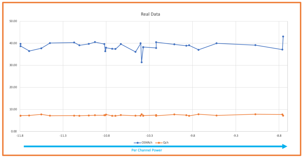
Collected from Real device for Reference
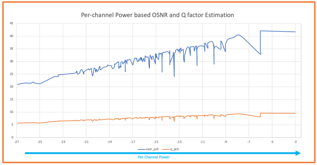
Calculated OSNR and Q factor based on Per Channel Power.
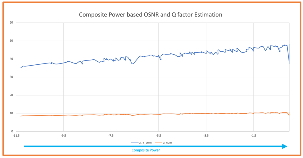 Calculated OSNR and Q factor based on composite Power.
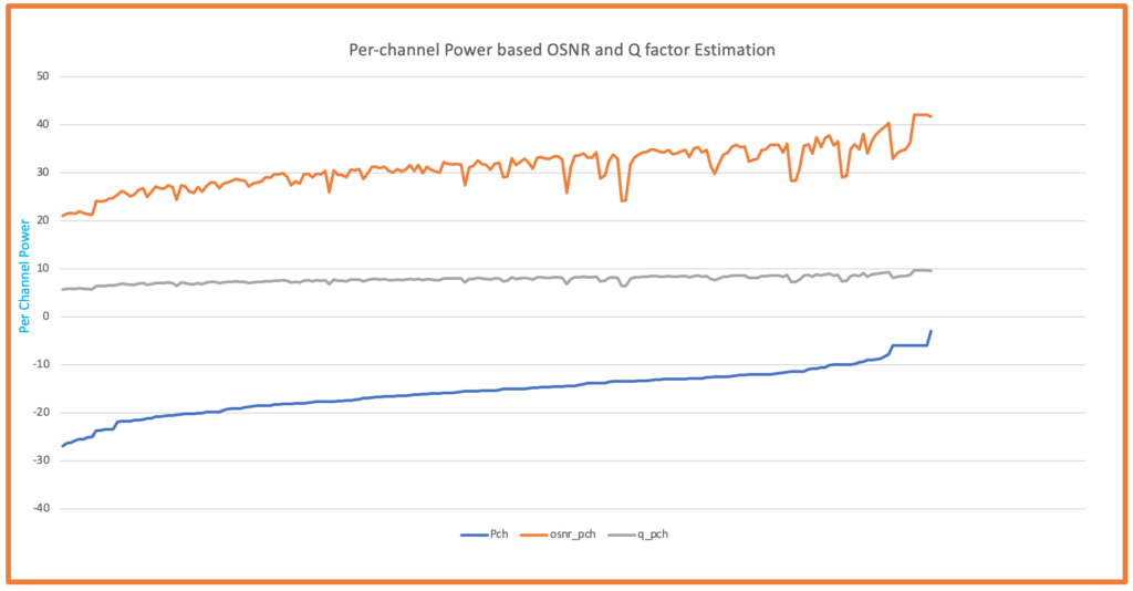
Calculated OSNR and Q factor based on Per Channel Power.
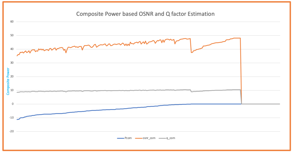
Calculated OSNR and Q factor based on composite Power.
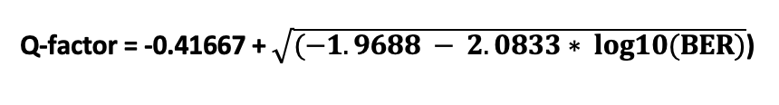
Formulas used for calculation of OSNR, BER and Q factor


Useful Python Script
import math
def calc_osnr(span_loss, composite_power, noise_figure, spans_count,channel_count):
"""
Calculates the OSNR for a given span loss, power per channel, noise figure, and number of spans.

Parameters:
span_loss (float): Span loss of each span (in dB).
composite_power (float): Composite power from amplifier (in dBm).
noise_figure (float): The noise figure of the amplifiers (in dB).
spans_count (int): The total number of spans.
channel_count (int): The total number of active channels.

Returns:
The OSNR (in dB).
"""
total_loss = span_loss+10*math.log10(spans_count) # total loss in all spans
power_per_channel = composite_power-10 * math.log10(channel_count) # add power from all channels and spans
noise_power = -58 + noise_figure # calculate thermal noise power
signal_power = power_per_channel - total_loss # calculate signal power
osnr = signal_power - noise_power # calculate OSNR
return osnr


osnr = calc_osnr(span_loss=23.8, composite_power=23.8, noise_figure=6, spans_count=3,channel_count=96)
if osnr > 8:
ber = 10* math.pow(10,10.7-1.45*osnr)
qfactor = -0.41667 + math.sqrt(-1.9688 - 2.0833* math.log10(ber)) # calculate OSNR
else:
ber = "Invalid OSNR,can't estimate BER"
qfactor="Invalid OSNR,can't estimate Qfactor"

result=[{"estimated_osnr":osnr},{"estimated_ber":ber},{"estimated_qfactor":qfactor}]
print(result)
Above program can be tested by using exact code at link.

 How to convert dBm to mW

