OSNR: What does this mean; Why do we need and How to take care of it?
A Comprehensive Guide to Understanding Optical Signal-to-Noise Ratio in Fiber Optic Communication Systems
Signal to Noise Ratio (SNR) is not an unknown terminology for Engineers and Tech professionals who are dealing with Digital or Analog form of Communication. Here we will explore the aspect of SNR in Optical Fiber Communication space known as Optical Signal to Noise Ratio (OSNR).
Warning! Keep patience while scrolling down to read as this article may seem long as this is important topic. Whole content is collected from free available trusted sources and can be downloaded or shared and covers content for everyone from beginner to professional so reader can absorb what he wants.
Bingo! Let's start it.
Some Handy Definitions of OSNR
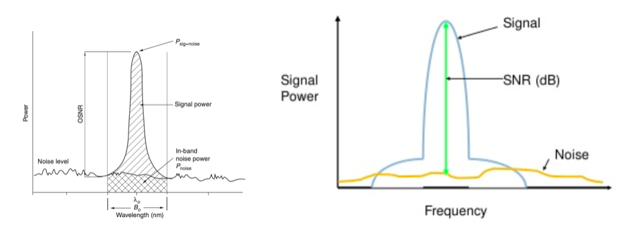
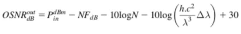
- OSNR [dB] is the measure of the ratio of signal power to noise power in an optical channel.
- OSNR is the short form of Optical Signal to Noise Ratio. It is key parameter to estimate performance of Optical Networks. It helps in BER calculation of Optical System.
- OSNR is important because it suggests a degree of impairment when the optical signal is carried by an optical transmission system that includes optical amplifiers.
- If we know the OSNR and the bandwidths, we can find Q and the BER.
- It can be seen as the QoS at the physical layer of optical networks. OSNR is directly related to bit-error rate, which will lead to packet losses seen by higher layers.
- OSNR indirectly reflects BER and can provide a warning of potential BER deterioration.
- OSNR has long been recognised as a key performance indicator for amplified high-speed transmission networks to ensure network performance and reliability and it is related to many design parameters such as number of repeaters/amplifiers, reach, available modulation formats etc.
- OSNR is a metric for the quality assessment of received signals that are corrupted by the ASE noise of EDFAs. OSNR is defined as the ratio of the average optical signal power to the average optical noise power.
Below are some visual representations showing OSNR concepts:
OSNR Calculation and Mathematical Formulas
For a single EDFA with the output power Pout and the noise power NASE, OSNR is computed as:
NFstage is the noise figure of the stage, h is Plank's constant (6.6260 × 10⁻³⁴), ν is the optical frequency 193 THz, and Δf is the bandwidth that measures the NF (it is usually 0.1 nm).
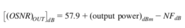
where:
- OSNRdB = optical signal to noise ratio of the optical amplifier, dB
- Pin.dBm = average amplifier input signal power (DWDM systems use single-channel power), dBm
- NF = amplifier noise figure, dB
- h = Planck's constant 6.626069 × 10⁻³⁴, Js
- f = signal center frequency, Hz
- Br = optical measurement bandwidth RBW, Hz
If the measurement optical bandwidth can be assumed to be 0.1 nm (12.48 GHz),
where:
- OSNRF.dB = final OSNR seen at the receiver, dB
- Psource.dBm = average source signal power into the first span (DWDM systems use single-channel power), dBm
- NF = amplifier noise figure, the same for all EDFAs, dB
- Br = optical measurement bandwidth, Hz
- N = number of amplifiers in the fiber link excluding the booster
- Γ = span loss, the same for all spans, dB
Important Note: Above equation provides the actual mathematical calculation of OSNR. This calculation method has quite a few approximations in which we can still find the system OSNR to a great degree of accuracy. In a multichannel WDM system, the design should consider OSNR for the worst channel (the one that has the worst impairment). The worst channel is generally the first or last channel in the spectrum.
We can see that the EDFA gain factor G is not considered. That is because OSNR is a ratio, and the gain acts equally on signal and noise, canceling the gain factor in the numerator and denominator. In other words, although EDFAs alleviate the upper bound on transmission length due to attenuation, by cascading EDFAs in a series, the OSNR is continuously degraded with transmission length and ASE (from EDFAs). This degradation can be lessened somewhat by distributed Raman amplifiers (DRAs).
Addition of Raman and OSNR Change
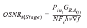
As we can see from above equation the factor GRA in the numerator actually enhances the OSNR of the system. (stages) could be considered as EDFA hops here.

OSNR-based design essentially means whether the OSNR at the final stage (at the receiver) is in conformity with the OSNR that is desired to achieve the required BER. This also guarantees the BER requirement that is essential for generating revenue.
OSNR Measurement in Modern Networks
Traditional Measurement Methods
This method works well for networks up to 10G, without any Reconfigurable Optical Add-Drop Multiplexers (ROADM).
But traditional way of measurement don't work anymore in High Speed Communications
However, IEC 61280-2-9 isn't feasible for 100G+ signals as well as ROADM networks.
Figure below illustrates 100G channels spaced 50GHz apart, which is a common spacing in modern submarine (and terrestrial) networks. Polarization-Multiplexed (Pol-Mux) 100G+ signals are typically wider (require more optical spectrum) than legacy On-Off-Keyed (OOK) 10G signals, meaning they could overlap with neighboring channels. Accordingly, the midpoint between channels no longer consists only of noise, but rather of signal plus noise. Thus, the IEC method applied to 100G+ Pol-Mux signals will therefore lead to an overestimation of noise and inaccurate measurement data leading to incorrect decisions.
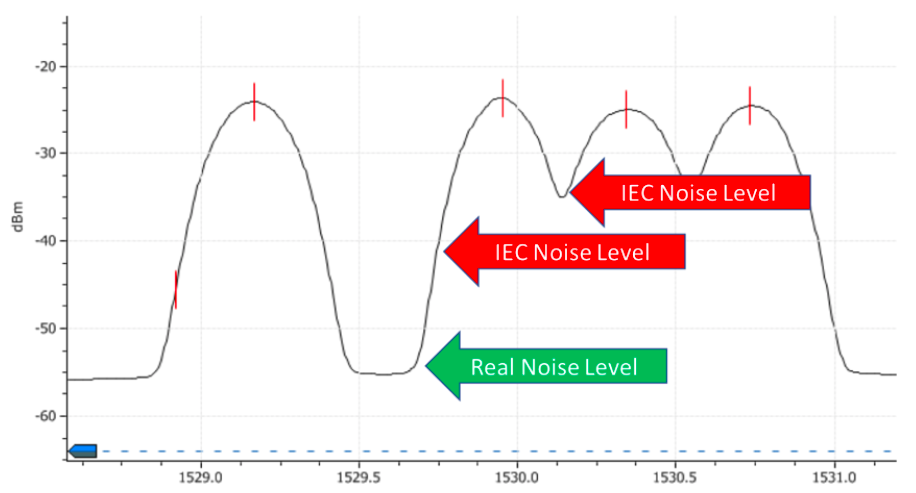
Figure: IEC 61280-2-9 Method Fails with Dense Pol-Mux 100G+ signals
Figure below illustrates a 100G signal that has gone through a ROADM, with the green area showing the channel bandwidth. Given filters inside a ROADM, the noise at the midpoint between channels will be carved (or filtered), leading to an underestimation of the noise level, if the IEC 61280-2-9 method is used, meaning this method is not feasible in ROADM-enabled coherent submarine networks.
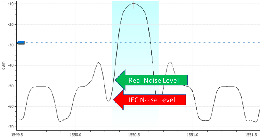
Figure: IEC 61280-2-9 Method Fails in ROADM 100G+ Pol-Mux Networks
To address the issues described above, in-band OSNR was introduced around 2009 to support OSNR measurements of 10G signals in ROADM networks and 40G OOK signals. However, this method can't be applied to coherent, Pol-Mux 100G+ signals, because of technical reasons beyond the scope of this blog. Consequently, Pol-Mux OSNR techniques have been introduced to support 100G+ signals, which is the topic of the latest standards.
Appropriate Standards for Pol-Mux OSNR Measurements
There are two standards providing relevant guidelines for OSNR measurements of Pol-Mux signals. They are the China Communications Standards Association (CCSA) YD/T 2147-2010 standard and the IEC 61282-12 standards, which was recently introduced in February 2016. Both standards provide a future-proof definition of OSNR, which can be applied to any type of signal, at any data rate, including super-channels and flexible-grid signals.
Specifically, the IEC-61282-12 standard specifies that:
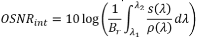
where:
- s(λ) is the time-averaged signal spectral power density, not including ASE, expressed in W/nm
- ρ(λ) is the ASE spectral power density, independent of polarization, expressed in W/nm
- Br is the reference bandwidth expressed in nm (usually 0.1nm if not otherwise stated)
- and the integration range in nm from λ1 to λ2 is chosen to include the total signal spectrum
Important Consideration: The only drawback of these two standards is that a careful application of their formulae requires turning off channels, to access the Amplified Spontaneous Emission (ASE) noise floor, which isn't possible on an in-service network lest we upset end-users! Fortunately, in-service Pol-Mux OSNR methods have been introduced.
OSNR Method Summary by Signal Type
| Data Rate | ROADM Present? | OSNR Method | Works on in-service network? |
|---|---|---|---|
| ≤10G signals | No | IEC 61280-2-9 | Yes |
| ≤10G signals | Yes | In-band OSNR | Yes |
| 100G+ Pol-Mux | No/Yes | Pol-Mux OSNR (IEC 61282-12 or CCSA YD/T 2147-2010) | Yes (with modern equipment) |
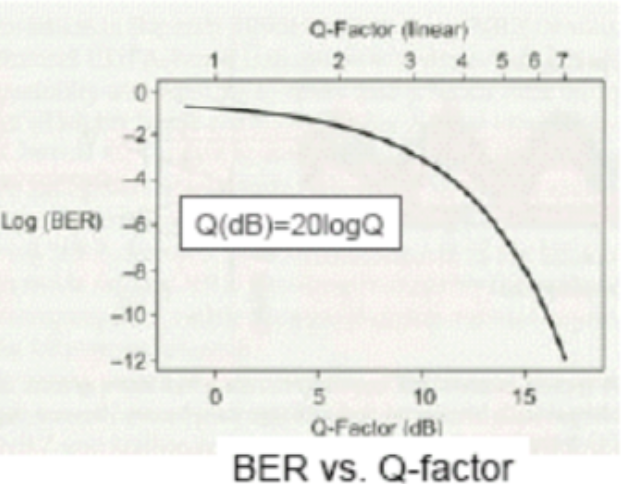
OSNR Relationship with BER and Q-Factor
The logarithmic value of Q (in dB) is related to the OSNR:
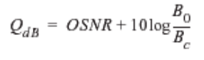
In the equation, B0 is the optical bandwidth of the end device (photodetector) and Bc is the electrical bandwidth of the receiver filter.
Key Insight: Q is somewhat proportional to the OSNR
BER Formulas for the Most Common QAM Systems
Gray coding is assumed for all formats.
For PM-BPSK the exact formula is:
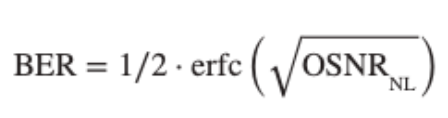
For PM-QPSK the exact formula is:
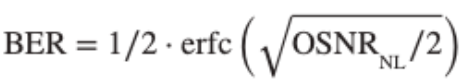
For PM-16QAM and PM-64QAM:
The following formulas are approximate, but their accuracy is better than ±0.05 dB of OSNRNL over the range 10-1 and 10-4:


EDFA Noise – Why Input Power Matters
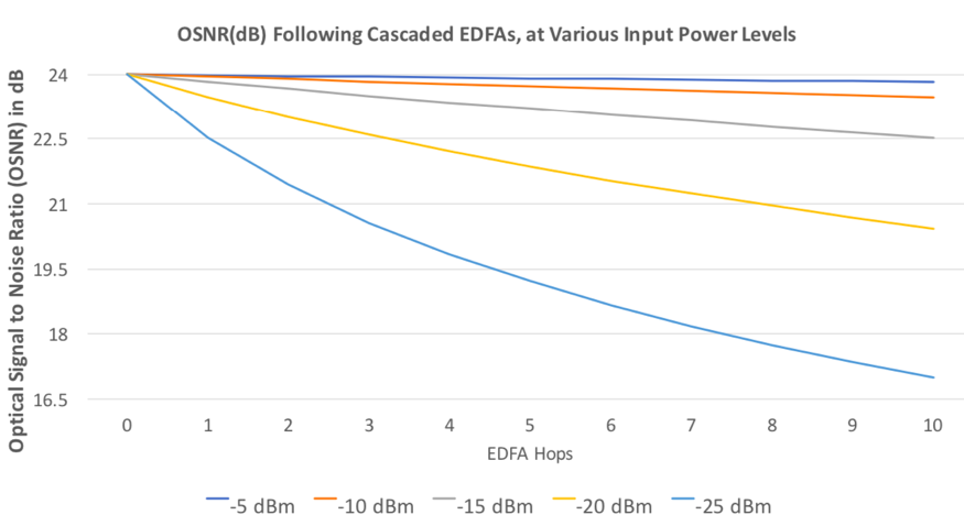
Optical signal suffers more than only attenuation. In amplitude, spectrally, temporally signal interaction with light-matter, light-light, light-matter-light leads to other signal disturbances such as:
- Power reduction
- Dispersion
- Polarization
- Unbalanced amplification
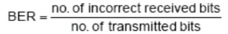
Thus leading to random noise, which causes misalignments, jitter and other disturbances resulting in erroneous bits, the rate of which is known as bit-error-rate.
Because of all possible influences outlined, bits transmitted by source and bits arriving at the receiver may not have the same value. In actuality a threshold value is set at the receiver, above the threshold refers to a logic "one" and below threshold refers to a logic "zero".
In order to measure BER in photonic regime, the optical signal is converted to electrical signal.
Example: Assuming a confidence level of 99%, BER threshold set at 10-10 and a bit rate of 2.5 Gb/s the required number n is 6.64 x 10¹⁰
Given the OSNR, the empirical formula to calculate BER for single fiber is:
Mathematical Example
Assume that OSNR = 14.5 dB
Then Log10(BER) = 10.7 - 1.45(14.5) = -10.30
Therefore BER = 10(-10.30)
BER is approximately 10-10
In an experimental environment where factors such as loss, dispersion, and non-linear effects are excluded, if the OSNR is less than the specified threshold, the pre-FEC BER will be excessively large and uncorrectable bit errors will be generated. The OSNR threshold in this case is called B2B OSNR tolerance.
Calculating OSNR from OSA (Optical Spectrum Analyzer)
As can be seen from the definitions above, two quantities must be known to compute OSNR: the Total Signal Power, and the amount of ASE Noise Power present in a 0.1nm bandwidth.
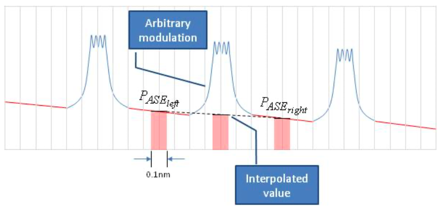
Measuring the ASE Power
When the ASE noise floor is clearly visible left and right of the optical signal, the ASE Noise Power at the signal wavelength can be interpolated from two measurements made left and right of the signal.
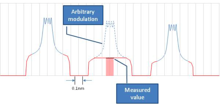
Alternately, when the noise floor is not visible left and right, the optical signal needs to be removed temporarily in order to allow the measurement of the ASE Noise Power at the signal wavelength.
- This is the case when some filtering devices implemented somewhere in line are removing some of the noise between channels (Example: WSS).
- This could also be the case if the modulated signal bandwidth is so large so that the tail of adjacent signals overlaps the open space between them – masking the noise floor.
Note: Power values are frequently provided in dBm by the OSA – whether the measurements is made using integrated power function or a user-specified resolution bandwidth. To convert the values in dBm to mW, the following relation must be used:
PmW = 10(PdBm/10)
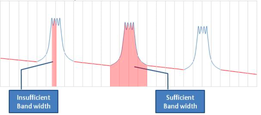
Measuring the Total Signal Power
When making this measurement it is important to use a bandwidth that is large enough to capture the entire signal:
- If using an OSA with variable resolution bandwidth, this means that the resolution bandwidth has to be set larger than the width of the signal.
- If using an integrated-power function between vertical markers, the markers have to be set to include the entire signal bandwidth.
Important Note: When measuring a DWDM spectrum, the power of each DWDM signal cannot be measured independent of ASE noise present in the measurement bandwidth.
I.e., the value that is actually measured is: Total Signal Power + ASE Noise Power
To get the Total Signal Power only, the ASE noise content (measured separately in the previous step) must be subtracted from the measurement. Since the measurement bandwidth used to measure the noise on its own (ASE BW) may be different from the bandwidth used to measure the signal (Signal BW), a factor is added to the equation. This removes the correct amount of noise from the measurement.
where:
- Signal BW is the bandwidth used to measured the signal
- ASE BW is the bandwidth used to measure the ASE Noise Power only (e.g., 0.1nm)
Calculating OSNR from Measurements
Since OSNR must be reported as signal power with respect to 0.1nm worth of ASE noise, the denominator of the OSNR equation also includes a factor. This adjusts the amount of ASE noise measured to an amount expected inside a 0.1nm bandwidth.
In a transmission chain, the relative evolution of the optical signal and noise levels is usually characterized by the optical signal-to-noise ratio (OSNR). The OSNR, in a given optical bandwidth, is defined as the ratio of signal power to noise power.
OSNR Requirements for Different Modulation Formats
The exact requirements at the receiver will vary from one manufacturer to another. The table below displays a few average OSNR figures to guarantee a BER lower than 10-8 at the receiver:
| Modulation Format | Required OSNR (dB) | Spectral Efficiency | Typical Application |
|---|---|---|---|
| OOK (On-Off Keying) | 12-14 dB | 0.4 b/s/Hz | Legacy 10G systems |
| QPSK | 10-12 dB | 2 b/s/Hz | Long-haul 100G |
| 16-QAM | 16-18 dB | 4 b/s/Hz | Metro 200G |
| 64-QAM | 22-24 dB | 6 b/s/Hz | Short-reach 400G |
Design Consideration: These values are approximate and depend on many factors including FEC overhead, symbol rate, and specific transceiver characteristics. Always refer to the specific equipment manufacturer's specifications for exact requirements.
Conclusion and Best Practices
Note: Now try to utilize the above concepts and equations whatever way you want.
Key Takeaways
- OSNR is a critical parameter for optical network design and performance monitoring
- Traditional measurement methods (IEC 61280-2-9) work well for legacy systems but fail for modern 100G+ networks
- Pol-Mux OSNR measurement techniques are essential for coherent transmission systems
- OSNR directly impacts BER and system performance
- Proper understanding of OSNR calculation helps in network planning and troubleshooting
- Different modulation formats require different OSNR levels for acceptable performance
- ROADM networks require special consideration for OSNR measurement
Practical Applications
Understanding OSNR is essential for:
- Network planning and dimensioning
- Amplifier placement and configuration
- Troubleshooting network performance issues
- Selecting appropriate modulation formats
- Validating system margins
- Commissioning and acceptance testing
Remember: OSNR is not just a number – it's a fundamental indicator of optical network health and a predictor of system performance. Regular monitoring and proper understanding of OSNR ensures reliable, high-quality optical transmission.
🎁 BONUS: Interactive OSNR Simulators
Experiment with these interactive tools to understand OSNR behavior in real optical networks!
Simulator 1: OSNR Calculator
Calculate OSNR based on input power and noise figure.
Results:
Simulator 2: BER vs OSNR Calculator
Calculate Bit Error Rate based on OSNR using the empirical formula: Log₁₀(BER) = 10.7 - 1.45(OSNR)
Calculated BER:
- BER < 10⁻¹² : Excellent
- BER = 10⁻⁹ to 10⁻¹² : Good
- BER = 10⁻⁶ to 10⁻⁹ : Acceptable (with FEC)
- BER > 10⁻⁶ : Poor (FEC may not correct)
Simulator 3: Multi-Span OSNR Degradation Visualizer
Visualize how OSNR degrades over multiple amplifier spans in a long-haul optical link.
System Status: Operational
Simulator 4: Modulation Format Selector
Determine the optimal modulation format based on available OSNR and desired reach.
Available Modulation Formats:
Recommended:
📊 Visual Reference Charts
OSNR Requirements by Modulation Format
ASE Noise Accumulation Visualization
Note: Each EDFA adds ASE noise, which accumulates through the chain. The green bars represent signal amplification, while the increasing light green area shows noise accumulation.