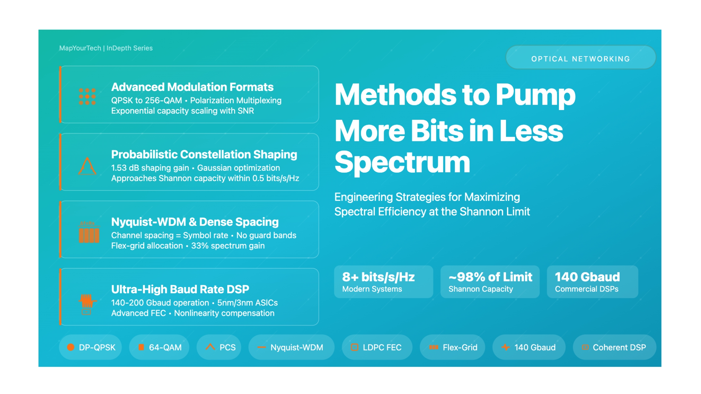

Methods to Pump More Bits in Less Spectrum in Optical Fiber
Engineering Strategies for Maximizing Spectral Efficiency at the Shannon Limit
Introduction: The Quest for Spectral Efficiency
The insatiable demand for bandwidth in optical fiber communications has driven engineers to develop increasingly sophisticated methods to transmit more data using less spectrum. As we approach the fundamental physical limits defined by Shannon's theorem and fiber nonlinearities, the focus has shifted from simply increasing power or bandwidth to intelligently optimizing every aspect of the transmission system.
Spectral efficiency (SE), measured in bits per second per Hertz (bits/s/Hz), has become the critical performance metric. Modern coherent optical systems have achieved spectral efficiencies exceeding 8 bits/s/Hz in laboratory demonstrations, representing a remarkable journey from the 0.4 bits/s/Hz of early 10 Gbps systems. This article explores the engineering methods enabling this transformation.
Why Spectral Efficiency Matters
With optical amplifier bandwidth fundamentally limited to approximately 4.8 THz in the C-band, and fiber capacity approaching theoretical maximums around 100 Tb/s per fiber, increasing spectral efficiency is the most practical path to higher capacities without deploying new fiber infrastructure. Every improvement in bits/s/Hz directly translates to increased network capacity using existing fiber plants.
Evolution of Spectral Efficiency in Optical Communications
Key Concepts: The Fundamentals of Spectral Efficiency
The Shannon Limit and Nonlinear Effects
The theoretical foundation for optical channel capacity begins with the Shannon-Hartley theorem, which defines maximum achievable data rate for a given bandwidth and signal-to-noise ratio:
Where C is capacity (bits/s), B is bandwidth (Hz), and SNR is the signal-to-noise ratio. For optical systems with polarization multiplexing, spectral efficiency becomes:
Where Rs is the symbol rate, Δf is the channel spacing, M is the number of constellation points, and r is the FEC overhead ratio.
However, optical fiber introduces a critical nonlinear constraint: the Kerr effect causes intensity-dependent refractive index changes, creating nonlinear noise that increases with signal power. This establishes the Nonlinear Shannon Limit, where adding more power or channels eventually produces diminishing or negative returns due to self-phase modulation (SPM), cross-phase modulation (XPM), and four-wave mixing (FWM).
Current State: Approaching the Limit
Modern commercial systems operate within 0.5-1.0 bits/s/Hz of the theoretical Shannon capacity. Laboratory demonstrations have achieved gaps as small as 3 dB from the Shannon limit, representing approximately 98% utilization of theoretical capacity. Further improvements require exponentially greater complexity for diminishing gains.
Spectral Efficiency Equation Components
To maximize spectral efficiency, engineers manipulate four primary variables:
- Symbol Rate (Rs): Higher baud rates directly increase throughput. Modern systems operate at 60-140 Gbaud, with next-generation DSPs targeting 200+ Gbaud.
- Channel Spacing (Δf): Reducing spacing packs more channels into available bandwidth. Nyquist-WDM achieves Δf = Rs (normalized spacing δf = 1), while super-Nyquist systems achieve δf < 1.
- Modulation Order (M): Higher-order formats (QPSK, 16-QAM, 64-QAM, 256-QAM) encode more bits per symbol but require exponentially higher SNR.
- FEC Overhead (r): Lower overhead increases net throughput but reduces error correction capability, requiring higher channel quality.
Practical Methods to Maximize Spectral Efficiency
1. Advanced Modulation Formats
Quadrature Amplitude Modulation (QAM)
QAM formats encode information in both the amplitude and phase of the optical carrier. Each symbol represents multiple bits, with M-QAM carrying log₂(M) bits per symbol. The evolution from QPSK (4-QAM) through 16-QAM, 64-QAM, to 256-QAM has driven spectral efficiency gains, but each doubling of constellation size requires approximately 6 dB more SNR.
QAM Constellation Diagrams
| Modulation Format | Bits/Symbol | OSNR Requirement | Typical Distance | Applications |
|---|---|---|---|---|
| DP-QPSK | 4 bits | 12-18 dB | 4,000-5,000 km | Ultra-long-haul, submarine |
| DP-16QAM | 8 bits | 20-25 dB | Several hundred km | Regional, 200G coherent |
| DP-64QAM | 12 bits | 24-28 dB | Up to 100 km | Metro DCI, 600G/800G |
| DP-256QAM | 16 bits | 32+ dB | <50 km | Short-reach DCI only |
Polarization Division Multiplexing (PDM)
PDM doubles capacity by transmitting independent data streams on orthogonal polarization states (X and Y polarizations). Combined with QAM, this creates formats like DP-QPSK (dual-polarization QPSK) and DP-64QAM. Modern coherent receivers use digital signal processing to separate and decode both polarizations simultaneously, effectively doubling spectral efficiency without requiring additional spectrum.
2. Probabilistic Constellation Shaping (PCS)
PCS represents one of the most sophisticated techniques for approaching Shannon capacity. The Shannon-Hartley theorem assumes signals with Gaussian probability distribution, but standard QAM uses all constellation points with equal probability, creating a uniform distribution. PCS bridges this gap by intelligently biasing transmission probabilities.
How PCS Works
Instead of transmitting all symbols equally, PCS makes low-energy inner constellation points more likely than high-energy outer points. This shapes the signal's probability distribution to approximate a Gaussian, providing up to 1.53 dB shaping gain over uniform QAM. This gain translates directly to extended reach or higher capacity.
PCS implementations use probabilistic amplitude shaping (PAS), which operates independently of forward error correction (FEC), allowing fine-grained rate adaptation. The modular architecture enables dynamic adjustment of the information rate while maintaining FEC coding gain, making it ideal for flexible optical networks that must adapt to varying channel conditions.
Benefits of PCS:
- Improved nonlinear tolerance: Lower average power reduces fiber nonlinear effects
- Fine rate granularity: Enables precise matching to channel capacity
- Extended reach: Shaping gain increases transmission distance by 10-20%
- Better channel utilization: Approaches Shannon limit more closely
3. Nyquist-WDM and Dense Channel Spacing
Traditional WDM systems leave significant guard bands between channels to prevent crosstalk. Nyquist-WDM dramatically improves spectral efficiency by reducing or eliminating these guard bands through precise spectral shaping.
Spectral Shaping Techniques
The ideal transmitted spectrum for maximum spectral efficiency is rectangular with bandwidth equal to the symbol rate Rs. This allows channel spacing (Δf) to equal the symbol rate, achieving the theoretical Nyquist limit where normalized spacing δf = Δf/Rs = 1.
WDM Channel Spacing Evolution
Implementation Approaches
Optical Nyquist-WDM
Uses optical filters (such as Waveshaper devices) to shape each channel's spectrum after modulation. Approximates rectangular spectral shape through precise optical filtering with high-frequency pre-emphasis. Successfully demonstrated in ultra-long-haul experiments with QPSK, 8QAM, and 16QAM formats.
Digital Nyquist-WDM
Applies digital filters (FIR filters with 32-600 taps) in the electrical domain before modulation. Uses digital-to-analog converters (DACs) to generate precisely shaped electrical signals driving the modulator. Enables real-time generation and offers greater flexibility for adaptive systems.
Modern systems achieve quasi-Nyquist operation with normalized spacing δf = 1.05-1.1, providing excellent spectral efficiency while avoiding the implementation complexity of perfect Nyquist filtering. This represents a practical balance between spectral efficiency and system robustness.
4. Orthogonal Frequency Division Multiplexing (OFDM)
Coherent optical OFDM (CO-OFDM) takes a fundamentally different approach to spectral efficiency. Rather than using a single carrier per channel, OFDM divides the channel bandwidth into many closely-spaced orthogonal subcarriers. This multicarrier approach offers several advantages:
- Inherent orthogonality: Subcarriers spaced at the symbol rate naturally avoid inter-symbol interference
- Superior CD/PMD tolerance: Lower symbol rate per subcarrier reduces dispersion effects
- Flexible bandwidth allocation: Individual subcarriers can be adaptively loaded
- Built-in spectral shaping: Rectangular spectra achieved through cyclic prefix
OFDM Variants for Different Applications
- No-Guard-Interval CO-OFDM: Eliminates spectral efficiency penalty from cyclic prefix, ideal for superchannels
- Reduced-Guard-Interval CO-OFDM: Balances efficiency and dispersion tolerance
- DFT-Spread OFDM: Reduces peak-to-average power ratio for better nonlinear tolerance
Laboratory demonstrations of CO-OFDM have achieved data rates exceeding 1 Tb/s over 600 km with spectral efficiencies comparable to or better than single-carrier systems. However, the high peak-to-average power ratio (PAPR) makes OFDM more sensitive to fiber nonlinearities, limiting its application in high-power long-haul systems.
5. Maximizing Symbol Rate (Baud Rate)
With modulation order limited by SNR requirements and channel spacing minimized through Nyquist techniques, increasing the symbol rate has become the primary method for capacity growth. Modern coherent DSPs operate at increasingly higher baud rates:
| Generation | Baud Rate | Technology Node | Typical Capacity | Commercial Status |
|---|---|---|---|---|
| Generation 1 | 28-32 Gbaud | 28nm | 100G-200G | Widely deployed |
| Generation 2 | 64-69 Gbaud | 16nm/7nm | 400G-600G | Current deployment |
| Generation 3 | 90-140 Gbaud | 7nm/5nm | 800G-1.2T | Shipping now (2024-2025) |
| Generation 4 | 150-200 Gbaud | 5nm/3nm | 1.6T-2.4T | Development/trials |
Engineering Challenges at High Baud Rates
- DAC/ADC bandwidth: Requires >100 GHz analog bandwidth with sufficient linearity
- DSP complexity: Equalization tap requirements scale with baud rate
- Power consumption: Higher processing rates demand advanced semiconductor nodes
- Component bandwidth: Modulators, drivers, and receivers must support wider bandwidths
The latest commercial DSPs from Acacia (Cisco) operate at 140 Gbaud, enabling 1.2 Tbps in a single pluggable module. Future roadmaps target 200 Gbaud and beyond, though each increase requires significant advances in analog-to-digital conversion, signal processing algorithms, and photonic integration.
6. Advanced Forward Error Correction (FEC)
FEC has evolved from simple Reed-Solomon codes to sophisticated soft-decision schemes approaching theoretical limits. Modern FEC techniques operate within 0.0045 dB of the Shannon limit for AWGN channels, representing nearly perfect utilization of available capacity.
Evolution of FEC Technology
- Hard-Decision FEC: Reed-Solomon, BCH codes with 7-20% overhead, operating at BER thresholds of 10⁻³ to 10⁻⁴
- Soft-Decision FEC: LDPC (Low-Density Parity-Check) and turbo codes with 15-27% overhead, operating at BER thresholds up to 2×10⁻²
- Spatially-Coupled LDPC: Latest generation achieving >30 dB net coding gain with 20% overhead
FEC Overhead Trade-off
Lower FEC overhead increases net spectral efficiency but requires higher pre-FEC SNR. Modern systems dynamically adjust FEC overhead based on measured channel quality, optimizing the trade-off between robustness and throughput. A reduction from 27% to 15% overhead improves net throughput by ~10%, but reduces error correction margin by several dB.
7. Digital Signal Processing Enhancements
Advanced DSP algorithms enable operation closer to theoretical limits by compensating for transmission impairments that would otherwise reduce spectral efficiency:
Critical DSP Functions:
- Chromatic Dispersion Compensation: Digital equalization using overlap frequency-domain techniques eliminates need for optical dispersion compensation
- Polarization Demultiplexing: Adaptive MIMO (multiple-input multiple-output) equalization tracks polarization rotation and separates X/Y polarizations
- Carrier Phase Recovery: Blind phase search (BPS) and other feedforward algorithms compensate for laser phase noise
- Nonlinearity Mitigation: Digital back-propagation (DBP) and perturbation-based methods partially compensate fiber Kerr nonlinearity
8. Flex-Grid and Elastic Optical Networks
Traditional optical networks divide spectrum into fixed 50 GHz or 100 GHz channels regardless of actual bandwidth requirements. Elastic Optical Networks (EON) with flex-grid technology represent a paradigm shift, enabling dynamic allocation of spectrum resources matched precisely to traffic demands.
The Flex-Grid Concept
Flex-grid networks define spectrum in fine granularity slots (typically 12.5 GHz as standardized by ITU-T G.694.1) rather than fixed channel widths. A connection can occupy any number of contiguous slots needed for its data rate, adapting the spectral occupancy to the actual requirement.
Fixed-Grid vs. Flex-Grid Comparison
Benefits of Flex-Grid Architecture
- Spectrum efficiency gain: 33% improvement when migrating from 50 GHz to 37.5 GHz effective spacing
- Right-sized channels: Allocate exactly the bandwidth needed (50G, 150G, 350G, etc.) rather than fixed increments
- Dynamic adaptation: Adjust channel bandwidth in response to traffic pattern changes
- Simplified network evolution: Accommodate multiple generations of equipment with different bandwidth requirements
Elastic Transponders and Rate Adaptation
Elastic transponders can dynamically adjust multiple transmission parameters to optimize performance:
Modulation Format Adaptation
Dynamically switch between QPSK, 8QAM, 16QAM, and 64QAM based on measured OSNR. For example, a transponder operating at 100 Gbps might use DP-QPSK for 2,000 km reach or switch to DP-16QAM for 500 km at higher spectral efficiency.
Symbol Rate Adaptation
Adjust baud rate to match required capacity and available spectrum. Operating at 32 Gbaud for 100G service saves power and spectrum compared to unnecessarily running at 64 Gbaud. Energy consumption scales with clock frequency.
Superchannels for High Capacity
Superchannels aggregate multiple closely-spaced subcarriers into a single logical channel, enabling terabit-scale capacity while simplifying network management. All subcarriers are added, routed, and dropped together as a single entity.
Superchannel Characteristics:
- Coherent aggregation: Multiple subcarriers (typically 3-10) with tight frequency locking
- Joint amplification: All subcarriers amplified together, simplifying power management
- Flexible bandwidth: 150 GHz to over 500 GHz total occupancy
- High capacity: 400G to 1.6T+ per superchannel in current deployments
- Network simplification: Treated as single routing entity despite multiple subcarriers
Practical Deployment Considerations
While flex-grid offers significant advantages, successful deployment requires: (1) Wavelength Selective Switches (WSS) with fine granularity and sharp filter edges to avoid crosstalk; (2) Software-defined control plane capable of routing and spectrum assignment (RSA) rather than traditional routing and wavelength assignment (RWA); (3) Guard bands between channels to compensate for real-world filter imperfections; and (4) Network management systems that can optimize spectrum allocation across multiple paths.
Energy Efficiency Benefits
Elastic networks deliver substantial energy savings through right-sizing:
- Modulation format adaptation enables skipping unnecessary regenerators on shorter links
- Symbol rate scaling reduces power consumption proportionally - 50% symbol rate reduction yields ~40% power savings in DSP and line cards
- Traffic-adaptive operation allows reducing capacity during off-peak hours, saving 20-32% energy in European-scale networks
- Putting spare protection equipment in low-power sleep mode until needed
Implementation Best Practices
System Design Considerations
1. Match Modulation Format to Link Budget
Select the highest-order modulation format sustainable by the available OSNR. Use adaptive modulation systems that can dynamically adjust format based on measured performance:
- Ultra-long-haul (>2,000 km): DP-QPSK or DP-8QAM with probabilistic shaping
- Long-haul (500-2,000 km): DP-16QAM with PCS
- Metro/regional (80-500 km): DP-16QAM to DP-64QAM
- Data center interconnect (<80 km): DP-64QAM to DP-256QAM
2. Optimize Channel Spacing vs. Nonlinearity
Tighter channel spacing improves spectral efficiency but increases crosstalk and nonlinear penalties. Use the GN model or enhanced GN model to predict optimal spacing:
- Start with quasi-Nyquist spacing (δf = 1.05-1.1) for most systems
- Monitor cross-phase modulation effects in high-capacity DWDM systems
- Consider flex-grid channel allocation to match traffic patterns
- Implement guard channels between high-power and sensitive channels
3. Power Optimization Strategy
Operate at the optimal launch power where linear SNR gains balance nonlinear penalties. This "sweet spot" varies by system configuration but typically occurs at:
- Long-haul systems: -2 to +2 dBm per channel
- Ultra-long-haul: -3 to 0 dBm per channel
- Metro systems: 0 to +3 dBm per channel
4. Measurement and Monitoring
Implement comprehensive performance monitoring to maintain optimal spectral efficiency:
- Monitor pre-FEC BER to detect degradation before service impact
- Track OSNR at multiple points in the optical path
- Measure frequency offset and polarization-dependent loss
- Use digital diagnostic features in coherent transceivers for real-time analysis
- Implement automated margin management to maximize capacity utilization
Common Pitfalls to Avoid
Overambitious Modulation
Using 64-QAM where 16-QAM is appropriate may reduce actual throughput due to higher BER and FEC overhead. Always verify adequate OSNR margin (typically 3-4 dB) before deploying higher-order formats.
Neglecting Nonlinear Effects
Tight channel spacing amplifies XPM and FWM. Use proper channel planning tools and validate system performance under full load before deployment. Empty channels don't reveal nonlinear problems.
Insufficient DSP Capability
Ensure coherent receiver DSP has adequate tap count for chromatic dispersion compensation at high baud rates. Undersized DSP limits achievable distances regardless of optical power budget.
Poor Spectral Hygiene
Amplifier gain flatness, filter concatenation, and WSS impairments accumulate across multiple spans. Implement spectral equalization and periodic optical regeneration to maintain signal quality.
Comprehensive Techniques Comparison
| Technique | SE Improvement | Complexity | Power Impact | Reach Impact | Deployment Status |
|---|---|---|---|---|---|
| High-Order QAM (16/64/256-QAM) |
2-4× over QPSK | High DSP | Increased | Reduced 50-90% | Widely deployed (16/64-QAM) |
| Polarization Multiplexing (PDM) |
2× capacity | Moderate DSP | Minimal increase | Neutral | Universal adoption |
| Probabilistic Shaping (PCS) |
1.53 dB SNR gain (~15% capacity) |
Moderate DSP | 10-15% reduction | Extended 10-20% | Gen 2/3 coherent |
| Nyquist-WDM (δf = 1.0-1.1) |
1.5-2× vs 50 GHz | High filtering | Minimal | Slight degradation | Common in metro/long-haul |
| Super-Nyquist WDM (δf < 1.0) |
2-2.5× vs 50 GHz | Very high DSP | Increased | Reduced | Laboratory/specialized |
| Coherent OFDM | 1.5-2× base rate | Very high DSP | High (PAPR) | Good CD/PMD tolerance | Niche applications |
| High Baud Rate (100-200 Gbaud) |
Linear with rate | High analog BW | Increased | Neutral to positive | Gen 3 coherent (140 Gbaud) |
| Advanced FEC (LDPC, SC-LDPC) |
Enables higher SE | Very high DSP | Increased 30-50% | Extended significantly | Universal in coherent |
| Flex-Grid/EON | 20-33% network gain | High control plane | 10-30% reduction | Adaptive per link | Growing deployment |
| Superchannels | Efficient >400G | Moderate | Optimized | Depends on format | Standard for 400G+ |
Strategy Selection Guidelines
- Maximum capacity, short distance (<100 km): 64-QAM/256-QAM + PCS + Super-Nyquist + High Baud Rate
- Balanced metro/regional (100-800 km): 16-QAM + PCS + Quasi-Nyquist (δf=1.05) + 90-140 Gbaud
- Long-haul optimization (800-2,500 km): 16-QAM/8-QAM + PCS + Standard spacing + Advanced FEC
- Ultra-long-haul (>2,500 km): QPSK + PCS + Moderate baud rate + Maximum FEC overhead
- Dynamic networks: Flex-grid + Elastic transponders with adaptive modulation and symbol rate
- High-capacity aggregation: Superchannels with optimized subcarrier spacing
Real-World Applications and Case Studies
Data Center Interconnect (DCI)
DCI represents the fastest-growing segment demanding maximum spectral efficiency. Hyperscale operators face exponential bandwidth growth driven by AI/ML workloads, requiring aggressive capacity scaling within existing fiber infrastructure.
Typical DCI Implementation
- Distance: 10-80 km between data centers
- Modulation: DP-16QAM to DP-64QAM with PCS
- Baud rate: 90-140 Gbaud
- Capacity: 400G-800G per wavelength, targeting 1.6T
- Channel spacing: 75-100 GHz (quasi-Nyquist)
- Spectral efficiency: 6-8 bits/s/Hz achieved
Success factors include excellent fiber quality (low PMD), high-performance DSPs with extensive equalization, and adaptive rate systems that maximize capacity for each link. Latest deployments use 800G ZR/ZR+ pluggables enabling router-to-router connectivity without external transponders.
Long-Haul Terrestrial Networks
Long-haul networks balance spectral efficiency against transmission distance, typically operating with moderate modulation orders to maintain reach while improving capacity beyond legacy 100G systems.
- Configuration: 80-100 km spans with EDFA amplification
- Modulation: DP-16QAM with probabilistic shaping
- Capacity: 200G-400G per wavelength over 1,000-2,000 km
- Spectral efficiency: 4-6 bits/s/Hz typical
- Key techniques: Soft-decision FEC, PCS, digital nonlinearity compensation
Submarine Cable Systems
Transoceanic cables prioritize reach over spectral efficiency but still employ advanced techniques to maximize capacity within OSNR constraints:
- Typical span: 50-60 km of ultra-low-loss fiber
- Modulation: DP-QPSK to DP-8QAM with extensive shaping
- Distance: 5,000-13,000 km
- Capacity: 150-250 Tbps per fiber pair (modern systems)
- Channel count: 100-200 wavelengths in C+L bands
Recent submarine systems use spatially-coupled LDPC codes, geometric constellation shaping, and advanced Raman amplification to achieve record capacities. The Atlantic 2 cable demonstrated >38 Tb/s over transoceanic distances using super-Nyquist spacing and 8QAM.
Performance Metrics and Testing
Key Performance Indicators
Proper measurement and monitoring of spectral efficiency systems requires tracking multiple interdependent metrics:
Primary Metrics
Spectral Efficiency (SE)
Definition: Net data rate divided by occupied bandwidth, measured in bits/s/Hz
Calculation: SE = (Rs × log₂(M) × 2) / (Δf × (1 + FEC_overhead))
Typical values: 2-4 bits/s/Hz (long-haul), 6-8 bits/s/Hz (metro/DCI)
Optical Signal-to-Noise Ratio
Definition: Ratio of signal power to ASE noise in reference bandwidth (typically 0.1 nm)
Measurement: OSA (Optical Spectrum Analyzer) at multiple points
Critical thresholds: 12-18 dB (QPSK), 20-25 dB (16-QAM), 24+ dB (64-QAM)
Secondary Metrics
| Metric | Description | Typical Range | Measurement Method |
|---|---|---|---|
| Pre-FEC BER | Bit error rate before error correction | 10⁻⁴ to 2×10⁻² | Coherent receiver DSP telemetry |
| Post-FEC BER | Bit error rate after FEC decoding | <10⁻¹⁵ (error-free) | External BER tester or telemetry |
| Q-Factor | Signal quality metric in dB | 8-15 dB typical | Derived from pre-FEC BER |
| EVM (Error Vector Magnitude) | Constellation accuracy metric | 10-30% typical | DSP constellation analysis |
| Chromatic Dispersion | Accumulated fiber dispersion | 0-200,000 ps/nm | DSP measurement or OTDR |
| PMD (Polarization Mode Dispersion) | Differential group delay | <10 ps for 100G+ | Specialized PMD analyzer |
| PDL (Polarization Dependent Loss) | Loss variation with polarization | <2 dB per element | PDL meter or DSP telemetry |
Testing Best Practices
System Characterization Tests
- Back-to-back testing: Establish baseline performance with minimal impairments (transmitter directly connected to receiver)
- Swept power testing: Vary launch power from -10 to +10 dBm to identify optimal operating point balancing linear SNR vs. nonlinearity
- Loading tests: Fully populate all WDM channels to verify crosstalk, XPM, and FWM effects under realistic conditions
- Dispersion tolerance: Test across expected CD and PMD ranges using emulation or actual fiber spans
- Margin testing: Verify adequate performance margin (typically 2-3 dB) above FEC threshold
Field Deployment Validation
Commissioning Procedure
After installation, validate each wavelength: (1) Measure OSNR at every amplifier site ensuring >3 dB margin above requirement; (2) Verify pre-FEC BER remains below 50% of FEC threshold (e.g., <1×10⁻² for 2×10⁻² threshold); (3) Test modulation format adaptation if equipped, confirming proper switching between formats; (4) Conduct 24-72 hour burn-in monitoring for errors and alarm conditions; (5) Perform controlled failover testing to verify protection switching.
Ongoing Monitoring Requirements
- Real-time telemetry: Continuous pre-FEC BER, OSNR, and CD tracking from coherent DSP
- Trend analysis: Identify degradation patterns indicating fiber cuts, component aging, or configuration changes
- Threshold alarms: Pre-FEC BER approaching FEC limit, OSNR drop >2 dB, sudden PDL increases
- Performance management: Automated systems to optimize launch power and modulation format based on measured conditions
Common Measurement Challenges
Spectral Overlap in Dense WDM
With Nyquist or super-Nyquist spacing, accurate OSNR measurement becomes difficult due to overlapping channel spectra. Solution: Use in-band OSNR measurement techniques via coherent receiver or polarization-nulling methods rather than traditional OSA interpolation.
Nonlinear Noise Characterization
Fiber nonlinearity creates signal-dependent noise that varies with traffic patterns. Solution: Test under full-load conditions with realistic traffic, use GN-model predictions validated against measurements, and maintain conservative power levels.
Key Takeaways
- Modern optical systems operate within 0.5-1 bits/s/Hz of Shannon capacity, representing ~98% utilization of theoretical limits
- Probabilistic constellation shaping provides up to 1.53 dB gain, enabling 10-20% reach extension or capacity improvement
- Nyquist-WDM with channel spacing equal to symbol rate maximizes spectral efficiency, achieving 6-8 bits/s/Hz in commercial systems
- Increasing baud rate (symbol rate) has become the primary capacity scaling method, with commercial systems now at 140 Gbaud targeting 200+ Gbaud
- Advanced FEC operating at 2×10⁻² pre-correction BER enables aggressive modulation formats while maintaining error-free transmission
- Higher-order QAM (64-QAM, 256-QAM) enables short-reach capacity but requires exponentially higher SNR: each doubling needs ~6 dB more OSNR
- Adaptive systems that dynamically optimize modulation, baud rate, and FEC overhead maximize spectral efficiency across varying channel conditions
- The nonlinear Shannon limit imposes a fundamental ceiling around 100 Tb/s per C-band fiber; future growth requires new fiber bands (L, S) or spatial multiplexing
Conclusion and Future Outlook
The methods to pump more bits into less spectrum have evolved into a sophisticated engineering discipline operating at the fundamental limits of physics. Through the combination of advanced modulation formats, probabilistic constellation shaping, Nyquist-WDM, ultra-high baud rates, and near-optimal FEC, modern optical systems achieve spectral efficiencies that seemed impossible just a decade ago.
However, we are approaching hard physical limits. With commercial systems already within 0.5 bits/s/Hz of the Shannon capacity and operating near the nonlinear Shannon limit for fiber, future gains will be increasingly difficult. The industry consensus suggests only 10-20% additional spectral efficiency improvement is achievable before hitting absolute physical barriers.
Future Directions
As single-fiber spectral efficiency plateaus, the next wave of capacity growth will come from:
- Spatial Division Multiplexing (SDM): Multi-core and multi-mode fibers to scale capacity through parallel spatial channels
- Extended spectral bands: Deployment of L-band (1565-1625 nm) and S-band (1460-1530 nm) amplification to double or triple available bandwidth
- Hollow-core fiber: Novel fiber designs with lower latency and potentially higher nonlinear thresholds
- AI-optimized DSP: Machine learning techniques for optimal constellation design and nonlinearity compensation
- Quantum-limited receivers: Phase-sensitive amplification approaching quantum noise limits
For network engineers and system designers, the practical message is clear: maximize spectral efficiency using proven techniques (PCS, Nyquist-WDM, adaptive modulation), but recognize that future capacity growth will increasingly depend on deploying additional fibers, extending to new spectral bands, or adopting spatial multiplexing technologies.
Quick Reference Guide
Spectral Efficiency Formula Reference
Where:
- SE = Spectral Efficiency (bits/s/Hz)
- Rs = Symbol Rate (Baud)
- Δf = Channel Spacing (Hz)
- M = Modulation Order (4 for QPSK, 16 for 16-QAM, 64 for 64-QAM, etc.)
- r = FEC Overhead Ratio (0.07 for 7%, 0.20 for 20%, etc.)
Common Configuration Examples
| Configuration | Parameters | Calculated SE | Net Rate (Gbps) |
|---|---|---|---|
| 100G Long-Haul | 32 Gbaud, DP-QPSK, 50 GHz, 20% FEC | 2.13 bits/s/Hz | 106.7 Gbps |
| 200G Regional | 64 Gbaud, DP-QPSK, 75 GHz, 15% FEC | 2.96 bits/s/Hz | 222 Gbps |
| 400G Metro | 64 Gbaud, DP-16QAM, 87.5 GHz, 15% FEC | 5.08 bits/s/Hz | 444 Gbps |
| 800G DCI | 90 Gbaud, DP-64QAM, 100 GHz, 20% FEC | 8.1 bits/s/Hz | 810 Gbps |
| 1.6T+ DCI (1.2T/1.6T is already proven between 2023-2025) | 140 Gbaud, DP-64QAM, 150 GHz, 15% FEC | 8.35 bits/s/Hz | 1.253 Tbps |
Troubleshooting Decision Tree
Low Spectral Efficiency Diagnosis
Symptom: SE below expected for configuration
- Check 1 - Channel Spacing: Verify Δf setting matches plan. Excessive spacing wastes spectrum.
- Check 2 - FEC Overhead: Confirm actual FEC matches design. Some systems auto-increase overhead degrading net rate.
- Check 3 - Modulation Format: Verify system is using expected format. May have downgraded due to low OSNR.
- Check 4 - Symbol Rate: Confirm actual baud rate. Some elastic transponders reduce rate in response to impairments.
High BER / Low OSNR Resolution
Symptom: Pre-FEC BER approaching threshold or OSNR <3 dB margin
- Action 1 - Power Optimization: Sweep launch power to find optimal point. May be too low (linear noise) or too high (nonlinear).
- Action 2 - Channel Loading: Temporarily disable adjacent channels to check XPM/FWM contribution.
- Action 3 - Filter Alignment: Verify WSS and ROADM filters properly centered on channel frequency.
- Action 4 - Format Change: If available, reduce modulation order (64-QAM → 16-QAM → QPSK) to gain margin.
- Action 5 - Add Regeneration: For fixed systems, consider optical or electrical regeneration at midpoint.
Industry Standards Reference
- ITU-T G.694.1: Spectral grids for WDM applications - defines flex-grid with 6.25 GHz granularity
- ITU-T G.709: Optical Transport Network (OTN) interfaces and rates
- IEEE 802.3: Ethernet standards including 400GbE and 800GbE
- OIF (Optical Internetworking Forum): 400ZR, 400ZR+, 800ZR specifications for pluggable coherent
- OpenROADM: Open specifications for ROADM architectures and operations
For educational purposes in optical networking and DWDM systems
Note: This guide is based on industry standards, best practices, and real-world implementation experiences. Specific implementations may vary based on equipment vendors, network topology, and regulatory requirements. Always consult with qualified network engineers and follow vendor documentation for actual deployments.

Optical Communications & Network Automation Expert | Author of 3 Books for Optical Engineers | Founder, MapYourTech
Optical networking engineer with nearly two decades of experience across DWDM, OTN, coherent optics, submarine systems, and cloud infrastructure. Founder of MapYourTech. Read full bio →
Follow on LinkedIn