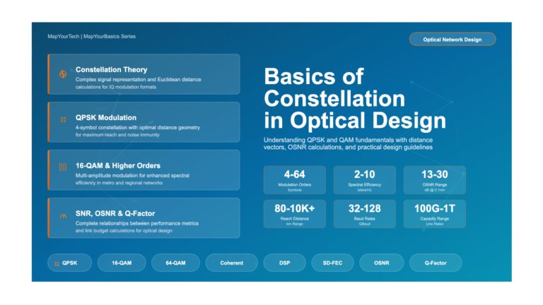
Basics of Constellation Diagrams in Optical Design: Understanding QPSK and QAM Fundamentals Basics of Constellation Diagrams in Optical Design: Understanding...
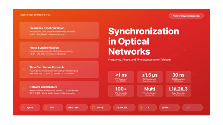
Synchronization in Optical Networks: A Comprehensive Deep Dive Synchronization in Optical Networks: A Comprehensive Deep Dive Exploring Frequency, Phase, and...
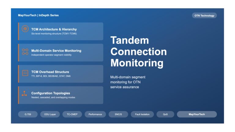
Tandem Connection Monitoring in OTN Networks | MapYourTech Tandem Connection Monitoring in Optical Transport Networks Comprehensive guide to multi-domain service...
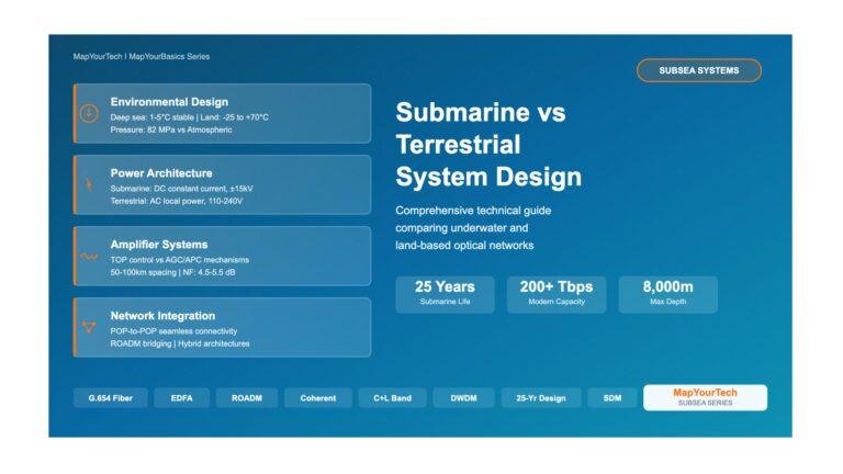
Submarine vs Terrestrial System Design Differences – Comprehensive Visual Guide Submarine vs Terrestrial System Design Differences Practical Information Based on...
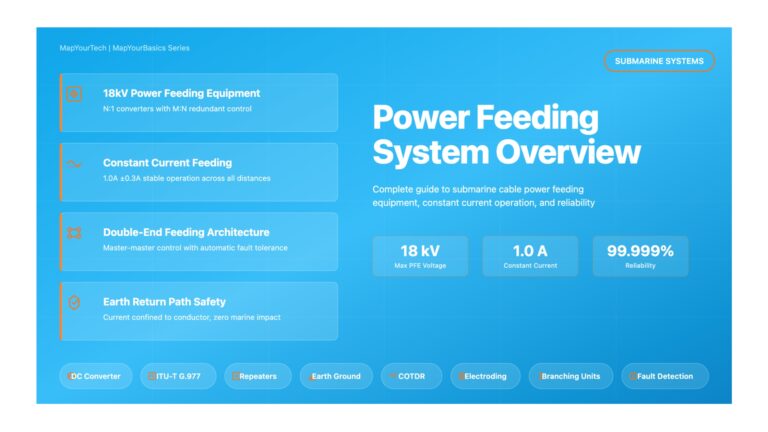
Power Feeding System Overview – Comprehensive Visual Guide Power Feeding System Overview Power Feeding Equipment (PFE) Practical Information Based on...
Submarine Cable Repair Operations – Comprehensive Visual Guide Overview of Submarine Cable Repair Operations Technical Guide Based on Industry Standards...