Timing vs Synchronisation in Telecommunication Networks
A Deep Dive into Modern Network Synchronization: Understanding Frequency, Phase, and Time-of-Day Requirements
1. Introduction
In modern telecommunication networks, the concepts of timing and synchronization are frequently used interchangeably, yet they represent distinct technical requirements with different implementation challenges and performance criteria. This confusion often leads to architectural errors, suboptimal network designs, and deployment failures that could have been avoided with a clear understanding of the fundamental differences between these concepts.
Synchronization, in its broadest sense, refers to the distribution of common frequency, phase, and time references across network elements to align their internal clocks and timing scales. Timing, conversely, typically refers to the absolute time-of-day information traceable to a recognized time standard such as Coordinated Universal Time (UTC). While all timing systems require synchronization, not all synchronization systems provide timing capabilities. This distinction becomes critical when designing networks for modern applications like 5G mobile systems, financial trading platforms, and power grid automation.
The evolution from legacy Time Division Multiplexing (TDM) networks to modern packet-based architectures has fundamentally transformed synchronization requirements. Traditional TDM systems like SDH and SONET required only frequency synchronization to prevent buffer slips and maintain circuit integrity. Modern applications, particularly Time Division Duplex (TDD) based mobile systems, demand microsecond-level phase alignment and nanosecond-level time-of-day accuracy to prevent radio interference and enable advanced features like carrier aggregation and coordinated multipoint transmission.
This deep dive examines the technical foundations, architectural implications, and practical deployment considerations for timing and synchronization in telecommunication networks. We explore the three fundamental dimensions of synchronization—frequency, phase, and time—and explain how different technologies address each dimension. The article provides comprehensive coverage of industry standards from ITU-T, IEEE, and IETF, along with real-world implementation guidance for network architects and engineers.
Understanding the distinction between timing and synchronization is not merely an academic exercise. The choice between Synchronous Ethernet (SyncE), Precision Time Protocol (PTP), Network Time Protocol (NTP), and Global Navigation Satellite System (GNSS) solutions directly impacts network performance, capital expenditure, operational complexity, and service reliability. Modern networks often require hybrid architectures that combine multiple synchronization technologies to meet diverse application requirements while maintaining cost efficiency and operational simplicity.
2. Historical Context
2.1 Legacy TDM Synchronization Era
The foundation of network synchronization was established in the TDM era when telephone networks required precise frequency alignment to prevent data loss. In SDH and SONET networks, synchronization meant frequency synchronization—ensuring all network elements operated at precisely the same clock rate. The ITU-T G.810 standard defined the fundamental architecture: a hierarchical distribution model where Primary Reference Clocks (PRCs) provided frequency references traceable to atomic standards, typically achieving accuracy better than 1×10-11.
TDM synchronization operated on straightforward principles. Network elements recovered the clock signal from incoming bit streams and used phase-locked loops to regenerate clean timing for outgoing transmissions. This physical-layer synchronization was deterministic, immune to packet delay variations, and provided exceptional stability. The Synchronization Status Message (SSM) mechanism, carried in SDH overhead bytes, allowed network elements to assess clock quality and select the best available reference source automatically.
The hierarchical TDM clock architecture defined distinct strata levels. G.811 specified PRC characteristics at the top tier, while G.812 defined Synchronization Supply Unit (SSU) specifications for distribution nodes, and G.813 covered SDH Equipment Clocks (SECs) at network edges. This architecture could support synchronization chains of up to 60 network elements (1 PRC, 20 SECs, 10 SSUs, etc.) while maintaining network-wide frequency accuracy within ±4.6 ppm under holdover conditions.
2.2 The Packet Network Transition
The migration to packet-switched networks—initially Ethernet and IP—eliminated the deterministic timing characteristics of TDM systems. Standard Ethernet allowed clock frequency tolerance of ±100 ppm between nodes, far exceeding TDM requirements. Early packet networks relied on external timing distribution (separate TDM networks or GPS receivers at each site), creating operational complexity and single points of failure.
The development of Synchronous Ethernet (SyncE), standardized in ITU-T G.8261/G.8262 series from 2006 onwards, addressed frequency synchronization in packet networks. SyncE applied TDM synchronization principles to Ethernet's physical layer, allowing frequency recovery from Ethernet line codes while maintaining packet data transparency. This innovation enabled migration from TDM to packet transport without sacrificing frequency synchronization quality.
However, SyncE solved only frequency synchronization. The emergence of mobile technologies requiring phase alignment—particularly CDMA2000, TD-SCDMA, and later LTE-TDD—created new challenges. Phase synchronization requires not just frequency alignment but also precise timing of signal transitions. A network might have perfect frequency synchronization (all clocks ticking at the same rate) but completely misaligned phases (clocks showing different times).
2.3 Emergence of Time-Critical Applications
The introduction of LTE-TDD in 2010 fundamentally changed synchronization requirements. TDD systems multiplex uplink and downlink signals on the same frequency by alternating time slots. Without precise time alignment between base stations (typically within 3 microseconds for small cells), transmissions from neighboring cells create severe interference patterns. One base station's downlink transmission during another's uplink reception slot causes what is known as base-station-to-base-station interference, degrading network capacity and coverage.
Beyond mobile networks, financial regulations like MiFID II mandated microsecond-level timestamp accuracy for trading systems. Power grid automation required sub-millisecond synchronization for phasor measurement units. Broadcast video production adopted IP-based workflows needing microsecond-level frame synchronization. Each application created specific timing requirements that existing synchronization technologies could not fully address.
These converging requirements drove development of the Precision Time Protocol (PTP), defined in IEEE 1588. Originally created for industrial automation, PTP was adapted for telecommunications through ITU-T telecom profiles: G.8265.1 for frequency synchronization, G.8275.1 for full on-path phase/time support, and G.8275.2 for partial network support. These profiles defined how to achieve nanosecond-level time distribution across packet networks despite variable packet delays.
2.4 The Modern Synchronization Landscape
Today's networks typically deploy hybrid synchronization architectures. SyncE provides stable frequency references at the physical layer, PTP distributes phase and time-of-day information at the packet layer, and GNSS receivers provide absolute UTC traceability at strategic network locations. The ITU-T G.827x series standards define how these technologies work together to meet application requirements ranging from 500 milliseconds (billing systems) to 130 nanoseconds (5G fronthaul relative timing).
The Enhanced Primary Reference Time Clock (ePRTC), specified in G.8272.1, represents the current state-of-the-art: combining GNSS receivers with autonomous atomic clocks to provide ±30 nanoseconds accuracy to UTC while maintaining performance during extended GNSS outages. This evolution reflects the industry's recognition that synchronization has become a critical network layer requiring the same redundancy and resilience as routing and switching infrastructures.
3. Core Concepts
3.1 The Three Dimensions of Synchronization
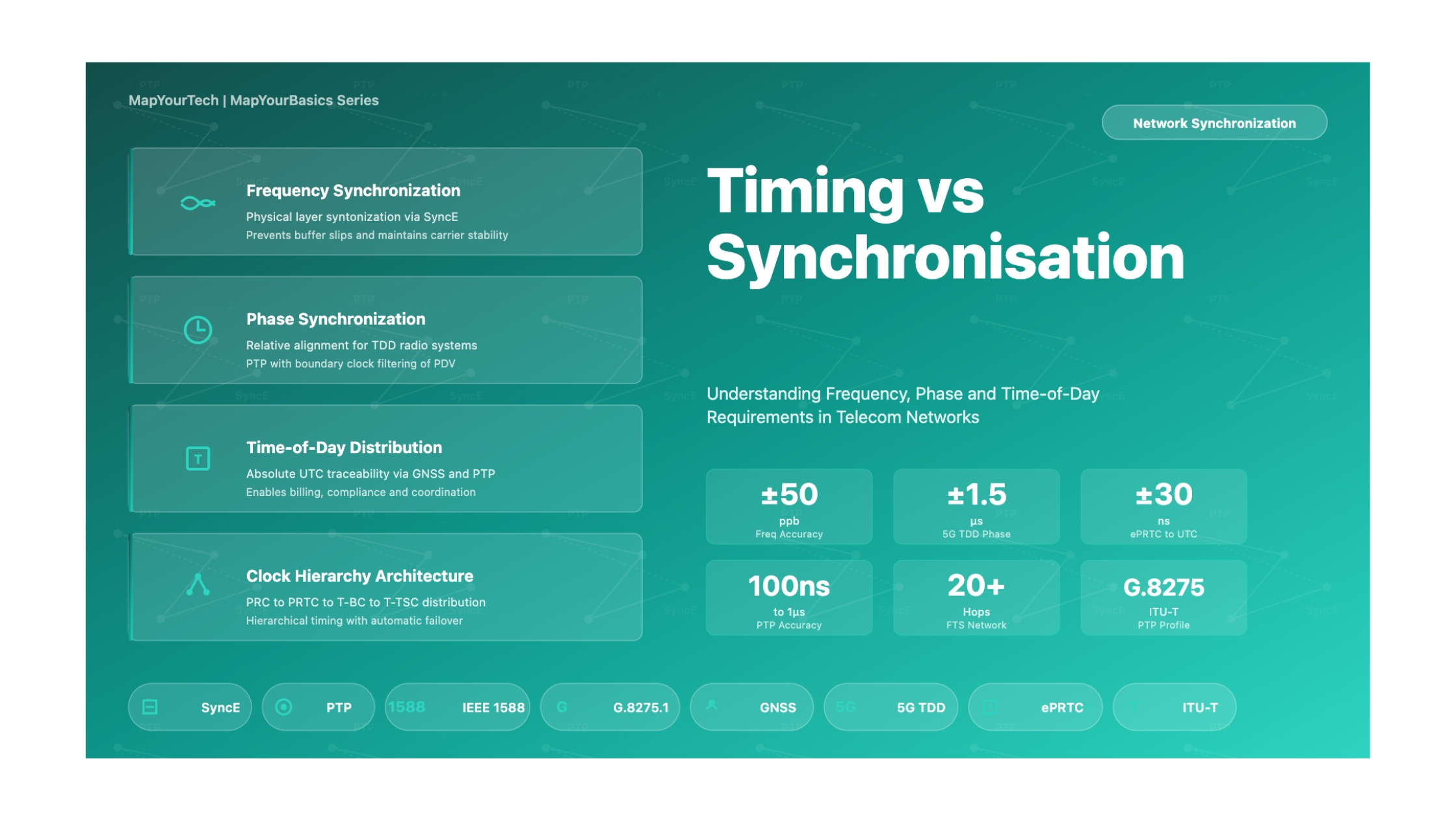
Understanding timing versus synchronization requires recognizing three distinct dimensions that networks must address: frequency synchronization (syntonization), phase synchronization, and time synchronization. Each dimension serves different purposes and requires different distribution technologies.
Frequency Synchronization
Frequency synchronization ensures all network clocks tick at precisely the same rate. If Clock A completes 1,000,000 cycles per second, Clock B must also complete 1,000,000 cycles per second within specified tolerance (typically measured in parts per billion, ppb). Frequency mismatches cause buffer overflows or underruns in TDM systems, leading to data slips—the insertion or deletion of entire frame structures.
Frequency Accuracy Formula:
Frequency Accuracy = |factual - fnominal| / fnominal

Where:
- factual = Measured clock frequency (Hz)
- fnominal = Target reference frequency (Hz)
- Result expressed in ppm (parts per million) or ppb (parts per billion)

Example:
For a 10 MHz clock with 0.05 Hz deviation:
Frequency Accuracy = 0.05 / 10,000,000 = 5 × 10-9 = 5 ppb
Phase Synchronization
Phase synchronization aligns the timing of signal transitions between clocks. Two clocks with identical frequencies can still be phase-misaligned—imagine two perfectly synchronized metronomes starting at different times. Phase error accumulates over time even with small frequency offsets. A 1 ppb frequency error creates approximately 1 microsecond of phase drift per 1000 seconds.
Phase synchronization is critical for TDD radio systems. Mobile base stations must transmit and receive in synchronized time slots. If one base station is transmitting while a nearby station is receiving, the transmitted signal creates interference. Phase alignment within 3 microseconds (LTE-TDD) or tighter tolerances (5G NR TDD requires 1.5 microseconds) prevents such interference patterns.
Time Synchronization (Time-of-Day)
Time synchronization provides absolute time-of-day information traceable to UTC. While phase synchronization requires relative alignment between network elements, time synchronization requires absolute accuracy to a recognized time standard. Applications include billing systems (100 milliseconds tolerance), network diagnostics (100 microseconds), and regulatory compliance (microsecond-level for financial systems).
The distinction between phase and time synchronization is subtle but important. Phase synchronization cares only about relative alignment—all network elements maintain consistent phase relationships. Time synchronization requires traceable accuracy to an external reference like UTC, typically provided by GNSS systems or national timing laboratories.
Figure 1: Three dimensions of synchronization with technology mapping and 5G TDD requirements
3.2 Timing Standards and Clock Hierarchy
Network synchronization relies on a hierarchical clock architecture where high-quality reference clocks distribute timing to lower-tier clocks. The ITU-T defines multiple clock specifications, each optimized for specific network positions and performance requirements.
Primary Reference Clocks (PRC and PRTC)
The Primary Reference Clock (G.811) represents the highest frequency accuracy achievable in networks, typically implemented with cesium atomic clocks or GNSS-disciplined oscillators. PRC frequency accuracy must be better than 1×10-11, equivalent to gaining or losing less than 1 second every 3,170 years. PRCs serve as the master frequency reference for entire synchronization networks.
The Primary Reference Time Clock (G.8272) extends PRC concepts to include time-of-day distribution. PRTC Class A provides ±100 nanoseconds accuracy to UTC, while PRTC Class B achieves ±40 nanoseconds. The Enhanced PRTC (G.8272.1) combines GNSS receivers with autonomous atomic clocks, providing ±30 nanoseconds accuracy while maintaining performance during extended GNSS outages lasting weeks.
Synchronization Supply Units and Equipment Clocks
Between PRCs at network cores and equipment clocks at network edges, intermediate synchronization nodes filter timing signals and provide holdover capability during reference failures. SSUs (G.812) and SECs (G.813) define performance requirements for these intermediate clocks. An SSU can maintain ±4.6 ppm frequency accuracy during 24-hour holdover periods when references are lost.
For packet networks, the Synchronous Ethernet Equipment Clock (EEC, G.8262) performs similar functions. EECs recover frequency from Ethernet physical layers and regenerate clean timing for downstream transmission. The enhanced EEC (eEEC, G.8262.1) provides improved performance for demanding applications like 5G fronthaul synchronization.
| Clock Type | Standard | Frequency Accuracy | Time Accuracy | Network Position | Typical Application |
|---|---|---|---|---|---|
| PRC | ITU-T G.811 | ±1×10-11 | N/A (frequency only) | Network core | SDH/SONET master, SyncE reference |
| PRTC Class A | ITU-T G.8272 | PRC equivalent | ±100 ns to UTC | Aggregation sites | PTP Grandmaster reference |
| PRTC Class B | ITU-T G.8272 | PRC equivalent | ±40 ns to UTC | Central offices | High-accuracy mobile timing |
| ePRTC | ITU-T G.8272.1 | PRC equivalent | ±30 ns to UTC | Critical hub sites | 5G core, resilient timing |
| SSU | ITU-T G.812 | ±4.6 ppm holdover | N/A | Distribution nodes | TDM timing distribution |
| EEC | ITU-T G.8262 | ±4.6 ppm holdover | N/A | Ethernet switches | SyncE networks |
| eEEC | ITU-T G.8262.1 | Enhanced holdover | N/A | Carrier Ethernet | 5G mobile backhaul |
| T-BC Class C | ITU-T G.8273.2 | Via SyncE/PTP | ±30 ns cTE | Aggregation switches | 5G fronthaul timing |
| T-BC Class D | ITU-T G.8273.2 | Via SyncE/PTP | ±5 ns cTE | High-precision nodes | Ultra-dense 5G, DCI timing |
3.3 Synchronization Metrics and Performance Measurement
Evaluating synchronization performance requires understanding several key metrics that characterize clock behavior and network timing quality. These metrics enable engineers to design networks meeting specific application requirements and diagnose timing failures.
Maximum Time Interval Error (MTIE)
MTIE measures the maximum peak-to-peak phase variation of a clock signal over specified observation intervals. For a perfect clock, MTIE would be zero at all observation intervals. Real clocks exhibit MTIE that increases with observation time due to frequency drift and environmental factors. ITU-T standards specify maximum MTIE values across observation intervals from 0.1 seconds to several days.
Time Deviation (TDEV)
TDEV characterizes timing signal stability by measuring time variations using a modified Allan deviation calculation. TDEV filtering removes frequency offset effects, making it particularly useful for characterizing wander performance. Unlike MTIE, which measures worst-case behavior, TDEV provides a statistical measure of timing quality averaging out short-term fluctuations.
Constant Time Error (cTE)
For PTP boundary clocks and transparent clocks, cTE quantifies the systematic time error introduced by clock processing. A Class C boundary clock must maintain cTE within ±30 nanoseconds. This specification ensures that timing degradation through network hops remains bounded, allowing calculation of maximum hop counts for given application requirements.
4. Technical Architecture
4.1 Synchronous Ethernet (SyncE) Architecture
Synchronous Ethernet brings physical-layer frequency synchronization to packet networks by modifying standard Ethernet to recover and distribute clock signals at the physical layer. Unlike standard Ethernet, which permits ±100 ppm clock variation between nodes, SyncE equipment synchronizes transmit clocks to received signals, creating frequency-synchronous Ethernet links throughout the network.
The SyncE architecture consists of several functional components. The Ethernet Equipment Clock (EEC) within each network element recovers the clock from incoming Ethernet signals using phase-locked loops. The recovered clock drives the transmit serializer, ensuring downstream equipment receives properly timed signals. This chain of clock recovery and retransmission distributes frequency from PRC sources throughout the network.
Quality traceability operates through the Ethernet Synchronization Messaging Channel (ESMC), specified in G.8264. ESMC uses Ethernet Slow Protocol frames to convey Synchronization Status Messages indicating clock quality levels. These messages allow automatic selection of the best available timing reference, similar to SSM operation in SDH networks. When multiple timing sources exist, network elements use ESMC quality levels to build loop-free timing trees.
Figure 2: Synchronous Ethernet architecture with EEC functional components and ESMC quality distribution
4.2 Precision Time Protocol (PTP) Architecture
The Precision Time Protocol provides phase and time-of-day synchronization across packet networks through exchange of timestamped messages between master and slave clocks. PTP operates at the application layer, making it media-agnostic but susceptible to packet delay variations that SyncE avoids. The ITU-T telecom profiles address these challenges through specific architectural choices and performance requirements.
PTP Clock Types and Hierarchy
PTP networks consist of several clock types forming a master-slave hierarchy. The Telecom Grandmaster (T-GM) clock provides the ultimate timing reference, typically receiving input from a PRTC. Boundary Clocks (T-BC) terminate PTP on incoming ports, recover timing, and generate new PTP messages on outgoing ports. Transparent Clocks (T-TC) forward PTP messages while measuring and compensating for residence time delays. Slave clocks (T-TSC) receive PTP messages and adjust local oscillators to match the master.
The distinction between Full Timing Support (FTS) and Partial Timing Support (PTS) architectures determines which clock types are deployed. G.8275.1 defines the FTS profile where every network element supports PTP and SyncE, using boundary clocks at each hop. G.8275.2 defines the PTS profile where PTP messages traverse some non-timing-aware network segments, placing greater burden on slave clock recovery algorithms to handle variable packet delays.
PTP Message Exchange
PTP synchronization relies on four message types exchanged between master and slave. Sync messages carry master timestamp T1. Follow_Up messages provide precise T1 values when hardware timestamping occurs after transmission. Delay_Request messages from slaves allow path delay measurement. Delay_Response messages return slave timestamp T4. By comparing these timestamps, slaves calculate offset from master and propagation delay, adjusting local clocks accordingly.
Hardware timestamping at the physical layer is critical for achieving sub-microsecond accuracy. Software timestamping introduces unpredictable latencies from operating system scheduling and protocol stack processing. Modern network interface cards and switches implement IEEE 1588 Hardware Timestamp Units that capture precise transmission and reception times at the PHY layer, minimizing timestamp uncertainty to nanoseconds.
PTP Offset and Delay Calculation:
Master-Slave Offset Calculation:

offset = [(T2 - T1) - (T4 - T3)] / 2

delay = [(T2 - T1) + (T4 - T3)] / 2

Where:
T1 = Master transmission timestamp (Sync message)
T2 = Slave reception timestamp (Sync message)
T3 = Slave transmission timestamp (Delay_Req message)
T4 = Master reception timestamp (Delay_Req message)

Example:
T1 = 1000.000000000 s
T2 = 1000.000002150 s
T3 = 1000.000005000 s
T4 = 1000.000007100 s

offset = [(2150 - 0) - (7100 - 5000)] / 2 = [2150 - 2100] / 2 = 25 ns
delay = [(2150 - 0) + (7100 - 5000)] / 2 = [2150 + 2100] / 2 = 2125 ns
4.3 Hybrid SyncE + PTP Architecture
Modern telecommunication networks typically deploy hybrid architectures combining SyncE for frequency and PTP for phase/time synchronization. This approach leverages SyncE's physical-layer stability while adding PTP's phase alignment capability. The combination achieves superior performance compared to either technology alone.
In hybrid deployments, SyncE provides a stable frequency reference to all network elements, eliminating frequency wander that would otherwise accumulate in pure PTP networks. PTP boundary clocks use the SyncE-derived frequency as their local oscillator reference, improving PTP recovery performance and reducing timing uncertainty. This synergy enables networks to achieve 10-100 nanosecond accuracy end-to-end across multiple hops.
The ITU-T G.8275.1 profile mandates this hybrid approach for Full Timing Support networks. Every network element must support both SyncE (with eEEC per G.8262.1) and PTP (with T-BC per G.8273.2). This ensures each hop contributes minimal timing degradation, allowing networks to scale to 20+ hops while maintaining sub-microsecond accuracy.
| Architecture Type | ITU-T Profile | Frequency Method | Phase/Time Method | Typical Accuracy | Deployment Scenario |
|---|---|---|---|---|---|
| Full Timing Support | G.8275.1 | SyncE (all hops) | PTP with T-BC | 100 ns - 1 μs | 5G fronthaul, new deployments |
| Partial Timing Support | G.8275.2 | Mixed (SyncE + non-sync) | PTP end-to-end | 1 μs - 10 μs | LTE backhaul, brownfield networks |
| Frequency Only | G.8265.1 | PTP or SyncE | Not applicable | ±50 ppb | FDD mobile, frequency services |
| GNSS Everywhere | N/A | GNSS direct | GNSS direct | 10 ns - 100 ns | Low-density sites with GPS visibility |
| Hybrid GNSS + PTP | G.8275.1 or G.8275.2 | SyncE primary, GNSS backup | PTP primary, GNSS backup | 10 ns - 1 μs | Critical services needing resilience |
5. Implementation Details
5.1 Network Design Considerations
Successful timing and synchronization deployment requires careful network design addressing reference clock placement, redundancy architecture, and failure recovery mechanisms. The network synchronization plan must align with application requirements while considering operational constraints and cost implications.
Clock Reference Placement Strategy
PRC and PRTC placement significantly impacts network performance and resilience. Centralized architectures place timing sources at core locations, distributing synchronization through hierarchical chains. This approach minimizes capital expenditure but creates potential bottlenecks and single points of failure. Distributed architectures deploy timing sources throughout the network, improving resilience but increasing costs and complexity.
For mobile networks, common practices include deploying PRTCs at regional aggregation sites serving clusters of cell sites. A typical tier-1 operator might maintain 10-20 PRTC locations nationwide, each feeding timing to 500-2000 base stations through SyncE and PTP distribution. Critical hub sites often deploy ePRTCs combining GNSS with atomic clocks, providing weeks of autonomous operation during satellite outages.
Redundancy and Protection Switching
Timing networks require redundancy mechanisms comparable to data plane protection. Each network element should receive timing from at least two independent sources, automatically switching to backup references upon primary failures. The ESMC protocol for SyncE and Best TimeTransmitter Clock Algorithm (BTCA) for PTP provide automatic reference selection based on quality indicators.
Protection architectures must avoid timing loops where clock signals inadvertently flow back toward their source, creating circular dependencies. Network design tools construct timing tree topologies ensuring loop-free distribution. When topology changes occur (link failures, maintenance events), the network must recompute valid timing paths without introducing loops or oscillations.
5.2 Mobile Network Specific Requirements
Mobile networks present unique synchronization challenges due to stringent radio interface requirements and geographic distribution of cell sites. Different mobile technologies impose varying synchronization requirements that network architects must understand and address.
LTE and 5G NR Synchronization
LTE FDD requires only frequency synchronization (±50 ppb) to maintain downlink and uplink carrier frequencies. LTE TDD additionally requires phase synchronization within ±1.5 microseconds for small cells to prevent base-station-to-base-station interference. 5G NR TDD tightens requirements further, demanding ±1.5 microseconds absolute accuracy plus ±130 nanoseconds relative timing between cooperating radio units for Coordinated Multipoint (CoMP) transmission.
These 5G requirements drive adoption of G.8275.1 Full Timing Support architectures with Class C or Class D boundary clocks. A typical 5G fronthaul segment might traverse 5-8 network hops from core to radio unit. Each hop must maintain constant time error within ±30 nanoseconds (Class C) or ±5 nanoseconds (Class D) to meet the cumulative ±130 nanoseconds budget.
| Mobile Technology | Frequency Requirement | Phase/Time Requirement | Typical Architecture | Critical Application |
|---|---|---|---|---|
| GSM | ±50 ppb (±100 ppb for pico) | None | SyncE or NTP | Handover support |
| UMTS FDD | ±50 ppb | None | SyncE | Carrier frequency accuracy |
| UMTS TDD | ±50 ppb | ±2.5 μs | SyncE + PTP or GPS | UL/DL slot alignment |
| CDMA2000 | ±50 ppb | ±3 μs to GPS time | GPS at cell sites | Soft handoff |
| LTE FDD | ±50 ppb | ±10 μs (for CDMA handover only) | SyncE | Frequency accuracy |
| LTE TDD | ±50 ppb | ±1.5 μs (small cell) / ±5 μs (large cell) | SyncE + PTP (G.8275.1/2) | Interference avoidance |
| 5G NR TDD | ±50 ppb | ±1.5 μs absolute, ±130 ns relative | G.8275.1 + eEEC + Class C/D BC | CoMP, carrier aggregation |
| 5G NR FDD | ±50 ppb | ±1.5 μs (for features requiring sync) | SyncE + PTP | Advanced features |
5.3 Monitoring and Troubleshooting
Operational networks require continuous monitoring of synchronization performance to detect degradations before they impact services. Modern network management systems collect timing metrics from distributed clock elements, analyzing trends and generating alarms for out-of-spec conditions.
Key Performance Indicators
Synchronization monitoring tracks several critical metrics. Clock quality indicators report whether each element remains locked to valid references. Phase error measurements quantify timing offset between local clocks and upstream references. Packet Delay Variation metrics for PTP networks identify network congestion affecting timing message delivery. Holdover performance tracking ensures backup clocks maintain acceptable accuracy during reference failures.
ESMC and PTP announce messages provide real-time quality information distributed through the network. Management systems correlate this protocol-level data with physical measurements, identifying discrepancies indicating equipment failures or configuration errors. Continuous monitoring enables proactive maintenance before timing degradations affect end services.
5.4 Migration Strategies
Transitioning from legacy synchronization architectures to modern packet-based timing requires careful migration planning. Brownfield deployments must maintain service continuity while incrementally introducing new technologies. Operators typically adopt phased approaches rather than wholesale replacements.
A common migration path starts with deploying SyncE throughout the transport network, providing frequency synchronization for existing TDM and mobile FDD services. Subsequently, PTP deployment begins at strategic locations supporting new TDD or 5G cell sites. The network operates in hybrid mode with both TDM and packet synchronization coexisting, gradually retiring TDM elements as services migrate to packet transport.
Migration complexity arises from ensuring timing continuity during transitions. Network segments may temporarily mix SDH, SyncE, and PTP synchronization with careful attention to clock selection and quality level mappings. Testing and validation at each migration phase prevents service impacts while building confidence in new architectures.
6. Performance Analysis
6.1 Timing Budget Analysis
Network timing budgets allocate allowable timing error across the synchronization chain from reference clock to end application. Each network element contributes some timing degradation through constant time error, dynamic time error, and noise generation. The cumulative effect must remain within application requirements.
Consider a 5G NR TDD deployment requiring ±130 nanoseconds relative timing between radio units. The timing budget might allocate: ±30 nanoseconds for the ePRTC/T-GM, ±10 nanoseconds per Class D boundary clock (assuming 5 hops = ±50 nanoseconds), ±30 nanoseconds for the radio unit's T-TSC, and ±20 nanoseconds margin for asymmetry and environmental factors. This yields ±130 nanoseconds total, meeting requirements with no margin for degradation.
Timing Budget Calculation:
Total Time Error = TEPRTC + Σ(cTEBC_i + dTEBC_i) + TETSC + TEasymmetry

Where:
TEPRTC = Primary reference time error (typically ±30 ns for ePRTC)
cTEBC_i = Constant time error of boundary clock i
dTEBC_i = Dynamic time error of boundary clock i
TETSC = Time slave clock recovery error
TEasymmetry = Path asymmetry contribution

Example for 5G Fronthaul (±130 ns requirement):
TEPRTC = ±30 ns (ePRTC per G.8272.1)
5 × cTEBC = 5 × (±5 ns) = ±25 ns (Class D BCs)
dTE contribution = ±20 ns (PDV effects)
TETSC = ±30 ns (Radio Unit clock)
TEasymmetry = ±15 ns (compensated fiber)
Total = 30 + 25 + 20 + 30 + 15 = ±120 ns (within ±130 ns budget)
6.2 Comparative Technology Performance
Different synchronization technologies exhibit distinct performance characteristics that influence architecture selection. Understanding these tradeoffs enables engineers to choose appropriate solutions for specific applications and network conditions.
SyncE provides exceptional frequency stability (equivalent to SDH synchronization) but cannot deliver phase or time-of-day information. PTP achieves nanosecond-level phase accuracy when deployed with proper boundary clock support but requires more complex network infrastructure and management. GNSS offers all three synchronization dimensions with high absolute accuracy but introduces single points of failure and vulnerability to jamming or spoofing attacks.
| Performance Metric | SyncE | PTP (G.8275.1) | PTP (G.8275.2) | GNSS Direct | NTP |
|---|---|---|---|---|---|
| Frequency Accuracy | ±50 ppb locked | ±50 ppb (via SyncE) | ±50 ppb (if SyncE used) | ±1 ppb | ±100 ppm |
| Phase Accuracy | N/A | 100 ns - 1 μs | 1 μs - 10 μs | 10 ns - 100 ns | N/A |
| Time-of-Day Accuracy | N/A | 100 ns - 1 μs | 1 μs - 10 μs | 10 ns - 100 ns to UTC | 1 ms - 10 ms |
| Holdover (24 hours) | ±4.6 ppm | Depends on EEC | Depends on oscillator | Depends on oscillator | Poor (>1 second) |
| PDV Sensitivity | Immune | Low (T-BC filtering) | High | N/A | Very High |
| Network Complexity | Low | High (all hops) | Medium | Very Low | Very Low |
| Maximum Hop Count | 20+ (G.803) | 20+ with Class C/D | Limited (5-10) | 1 (direct) | Limited |
| CAPEX per Node | Low | Medium-High | Low-Medium | Medium (GNSS receiver) | Very Low |
| Jamming/Spoofing Risk | None | None | None | High | None |
6.3 Packet Delay Variation Impact
Packet Delay Variation (PDV) represents the primary challenge for packet-based timing protocols like PTP and NTP. PDV occurs when timing packets experience variable queuing delays in network switches and routers due to traffic congestion, buffer management policies, and priority handling. These variations introduce noise into timing measurements that slave clocks must filter.
The magnitude of PDV depends on network loading and architecture. Well-engineered networks with strict Quality of Service (QoS) policies, priority queuing for PTP traffic, and minimal congestion can maintain PDV below 100 nanoseconds. Heavily loaded networks without proper QoS can exhibit PDV of milliseconds, making accurate timing recovery impossible without extensive filtering or deployment of boundary clocks.
G.8275.1 Full Timing Support architecture mitigates PDV through boundary clocks that terminate PTP on each hop. Each T-BC recovers timing, filters incoming PDV, and generates clean PTP messages for the next segment. This hop-by-hop recovery prevents PDV accumulation, enabling accurate end-to-end timing even across congested network segments. G.8275.2 Partial Timing Support requires more sophisticated slave clock algorithms to handle accumulated PDV effects.
Figure 3: Packet Delay Variation impact on timing accuracy with boundary clock mitigation strategy
7. Case Studies
7.1 5G Mobile Operator Synchronization Deployment
A major European mobile operator deployed 5G NR TDD services across 15,000 cell sites requiring precise synchronization for fronthaul and midhaul networks. The deployment demonstrates practical application of ITU-T G.8275.1 Full Timing Support architecture in a large-scale commercial network.
Architecture Design
The operator established 12 regional PRTC sites equipped with ePRTCs combining Galileo GNSS receivers with atomic oscillators. Each ePRTC site serves as master timing source for 1,200-1,500 cell sites through hierarchical distribution. The core transport network deployed SyncE across all optical Ethernet links, ensuring frequency synchronization independent of PTP performance.
PTP distribution uses Telecom Grandmaster clocks at ePRTC sites and Class C boundary clocks at aggregation switches. The network maintains timing chains typically 5-8 hops from T-GM to radio unit. Hardware timestamping on all network elements minimizes timestamp uncertainty to nanosecond levels. Dedicated PTP VLANs with strict priority queuing prevent packet delay variations exceeding 200 nanoseconds.
Challenges and Solutions
Initial deployment encountered fiber asymmetry issues where transmit and receive paths traversed different fiber routes. Testing revealed asymmetries up to 3 microseconds on some paths, exceeding the ±130 nanosecond relative timing budget by orders of magnitude. The operator implemented automated asymmetry measurement using calibration procedures at boundary clocks, storing corrections in network management systems.
GNSS jamming incidents at urban cell sites motivated deployment of holdover monitoring and automatic failover to network-based timing. The ePRTC atomic oscillators maintain ±1 microsecond accuracy for 72 hours during GNSS outages, preventing service impacts. Enhanced monitoring systems detect jamming within 60 seconds and alert operations teams for investigation.
Results
Post-deployment measurements confirm end-to-end timing accuracy between 80-150 nanoseconds across 95% of paths, well within the ±130 nanosecond requirement. The network supports 5G features including carrier aggregation and coordinated multipoint transmission without timing-related performance degradation. Operational availability exceeds 99.99% with no timing outages causing service impacts in the first year.
7.2 Financial Trading Platform Timestamp Accuracy
A financial services firm implemented microsecond-accurate timestamping for algorithmic trading systems to comply with MiFID II regulations requiring ±100 microsecond accuracy to UTC. The deployment illustrates stringent timing requirements in financial applications and regulatory compliance verification.
The architecture deployed PRTC Class B clocks at two geographically diverse data centers, each receiving GNSS timing from multiple satellite constellations. PTP distributes time-of-day to trading servers using G.8275.1 profiles with hardware timestamping on all network interface cards. Network Time Security (NTS) provides cryptographic authentication of timing sources, preventing spoofing attacks.
Continuous monitoring systems record all timestamps with audit trails demonstrating compliance. During one incident, a fiber cut disrupted connectivity to the primary PRTC site. The secondary site's PRTC maintained service with no accuracy degradation, and trading operations continued without impact. Regulatory audits confirmed sustained compliance throughout the event.
7.3 Power Grid Synchrophasor Deployment
An electric utility deployed synchrophasor measurement units across a regional transmission grid requiring sub-millisecond time synchronization for real-time grid state estimation. The project demonstrates timing requirements in critical infrastructure applications beyond telecommunications.
Phasor Measurement Units (PMUs) installed at 85 substations require ±1 microsecond time accuracy for proper phasor angle calculation. The utility's fiber optic communications network provides timing distribution using G.8275.2 Partial Timing Support, as not all intermediate switches support PTP boundary clocks. Local GNSS receivers at each substation provide backup timing sources.
The dual-path architecture (network PTP plus local GNSS) ensures timing continuity during network or satellite outages. Testing confirmed the system maintains accuracy requirements during simulated failure scenarios. The synchrophasor data enables real-time monitoring of grid conditions and early detection of instabilities, enhancing grid reliability and resilience.
8. Future Directions
8.1 Enhanced Timing Technologies
The synchronization field continues evolving to address emerging application requirements and technological advances. Several developments promise to enhance timing capabilities and resilience in future networks.
White Rabbit technology, standardized as IEEE 1588-2019 High Accuracy profile, achieves sub-nanosecond synchronization over optical fiber networks. By combining hardware timestamping, precise delay measurement, and physical layer integration, White Rabbit enables timing applications previously requiring direct connections to atomic clocks. Research facilities and advanced manufacturing environments are early adopters, with potential expansion to telecommunications applications requiring extreme accuracy.
Chip-scale atomic clocks reduce size and power consumption of atomic oscillators, enabling deployment at cell sites and edge locations. These miniature atomic clocks provide holdover performance measured in weeks rather than hours, dramatically improving resilience to GNSS outages. As costs decrease, widespread deployment becomes economically viable for critical timing applications.
8.2 5G Advanced and 6G Requirements
5G Advanced features in 3GPP Release 18 and beyond introduce even more stringent synchronization requirements. Joint communication and sensing applications, integrated sensing and positioning services, and extended reality services demand timing accuracy approaching 10 nanoseconds with extremely low latency variations. These requirements drive adoption of Class D boundary clocks and enhanced PRTC deployments.
6G research envisions terahertz communications, quantum key distribution integration, and pervasive artificial intelligence requiring unprecedented synchronization precision. Preliminary studies suggest requirements in the single-digit nanosecond range for certain applications. Achieving such performance at scale necessitates fundamental advances in synchronization architectures, likely combining optical frequency combs, quantum clocks, and distributed coherent timing networks.
8.3 Security and Resilience
Growing awareness of GNSS vulnerabilities drives development of resilient timing architectures less dependent on satellite signals. Coherent network PRTC (cnPRTC) specifications in G.8272.2 enable coordinated timing across multiple atomic clock sites, maintaining nanosecond accuracy even during complete GNSS loss. These systems compare clocks using high-precision network measurements, detecting anomalies and failures automatically.
Network Time Security (NTS) protocols add cryptographic authentication to timing distribution, preventing spoofing attacks. Future standards may mandate timing authentication for critical infrastructure applications. Research into quantum-resistant timing protocols prepares for post-quantum cryptography transitions.
8.4 Artificial Intelligence Integration
Machine learning algorithms increasingly optimize synchronization networks by predicting failures, identifying optimal clock sources, and compensating for environmental effects. AI-driven network management systems analyze timing metrics across thousands of nodes, detecting subtle degradations before they impact services.
Neural network-based clock recovery algorithms improve PTP slave performance in challenging network conditions. By learning patterns in packet delay variations, these algorithms filter noise more effectively than traditional algorithms, extending the reach of packet-based timing into previously unsuitable networks.
9. Conclusion
The distinction between timing and synchronization is fundamental to understanding modern telecommunication network requirements. Synchronization encompasses three dimensions—frequency, phase, and time-of-day—each requiring specific technologies and architectures to deliver. Timing refers specifically to absolute time-of-day information traceable to recognized standards like UTC.
Legacy networks required only frequency synchronization to prevent data slips in TDM systems. Modern applications, particularly mobile technologies like 5G TDD, financial systems, and smart grid infrastructure, demand precise phase alignment and nanosecond-level time accuracy. Meeting these requirements necessitates hybrid architectures combining Synchronous Ethernet for physical-layer frequency stability, Precision Time Protocol for phase and time distribution, and GNSS for UTC traceability.
Successful implementation requires careful attention to network design, timing budgets, redundancy architectures, and continuous monitoring. The ITU-T G.827x series standards provide comprehensive frameworks for packet network synchronization, defining clock specifications, network limits, and PTP profiles. Engineers must understand these standards and apply them appropriately for specific deployment scenarios and application requirements.
As networks evolve toward 5G Advanced and 6G, synchronization requirements will only increase in stringency. Future architectures must deliver higher accuracy, improved resilience, and enhanced security while maintaining operational simplicity and cost-effectiveness. The synchronization field continues advancing through technologies like chip-scale atomic clocks, quantum time distribution, and AI-driven optimization, ensuring network timing keeps pace with application demands.
Organizations deploying modern telecommunication networks must recognize synchronization as a critical infrastructure layer deserving investment and engineering attention comparable to routing and switching systems. Proper synchronization architecture prevents service degradations, enables advanced features, ensures regulatory compliance, and provides foundation for future technology adoption. Understanding timing versus synchronization is the first step toward building networks ready for tomorrow's applications.
Summary - Key Takeaways
- Synchronization has three distinct dimensions: frequency (syntonization), phase alignment, and time-of-day (absolute timing to UTC)
- SyncE provides TDM-grade frequency synchronization but cannot deliver phase or time information; PTP provides phase and time but requires careful network design
- Modern mobile networks (5G TDD) require hybrid architectures combining SyncE frequency stability with PTP phase distribution, achieving 100 ns to 1 μs accuracy
- Clock hierarchy spans from atomic PRTCs (±30 ns) through boundary clocks (±5 ns to ±30 ns cTE) to slave clocks, with cumulative errors bounded by timing budgets
- Packet Delay Variation is the primary challenge for packet-based timing; G.8275.1 Full Timing Support mitigates PDV through hop-by-hop boundary clock filtering
- Network resilience requires multiple timing sources, automatic failover mechanisms, and holdover capability—ePRTCs maintain specification for weeks during GNSS outages
10. References
- ITU-T Recommendation G.8271/Y.1366 – Time and phase synchronization aspects of telecommunication networks
- ITU-T Recommendation G.8275.1/Y.1369.1 – Precision time protocol telecom profile for phase/time synchronization with full timing support from the network
- ITU-T Recommendation G.8275.2/Y.1369.2 – Precision time protocol telecom profile for phase/time synchronization with partial timing support from the network
- ITU-T Recommendation G.8261/Y.1361 – Timing and synchronization aspects in packet networks
- ITU-T Recommendation G.8262 – Timing characteristics of synchronous equipment clocks
- ITU-T Recommendation G.8262.1 – Timing characteristics of enhanced synchronous equipment clocks
- ITU-T Recommendation G.8264 – Distribution of timing information through packet networks
- ITU-T Recommendation G.8272/Y.1367 – Timing characteristics of primary reference time clocks
- ITU-T Recommendation G.8272.1 – Timing characteristics of enhanced primary reference time clocks
- ITU-T Recommendation G.8273.2 – Timing characteristics of telecom boundary clocks and telecom time slave clocks
- ITU-T Recommendation G.811 – Timing characteristics of primary reference clocks
- IEEE Standard 1588-2019 – Standard for a Precision Clock Synchronization Protocol for Networked Measurement and Control Systems
- 3GPP TS 36.133 – Evolved Universal Terrestrial Radio Access (E-UTRA); Requirements for support of radio resource management
- 3GPP TS 38.133 – NR; Requirements for support of radio resource management
- MEF 22.2.1 – Mobile Backhaul Implementation Agreement – Phase 3
- RFC 5905 – Network Time Protocol Version 4: Protocol and Algorithms Specification
Recommended Reading:
Sanjay Yadav, "Optical Network Communications: An Engineer's Perspective" – Bridge the Gap Between Theory and Practice in Optical Networking
Developed by MapYourTech Team
For educational purposes in Optical Networking Communications Technologies
Note: This guide is based on industry standards, best practices, and real-world implementation experiences. Specific implementations may vary based on equipment vendors, network topology, and regulatory requirements. Always consult with qualified network engineers and follow vendor documentation for actual deployments.
Feedback Welcome: If you have any suggestions, corrections, or improvements to propose, please feel free to write to us at [email protected]

Optical Communications & Network Automation Expert | Author of 3 Books for Optical Engineers | Founder, MapYourTech
Optical networking engineer with nearly two decades of experience across DWDM, OTN, coherent optics, submarine systems, and cloud infrastructure. Founder of MapYourTech. Read full bio →
Follow on LinkedIn