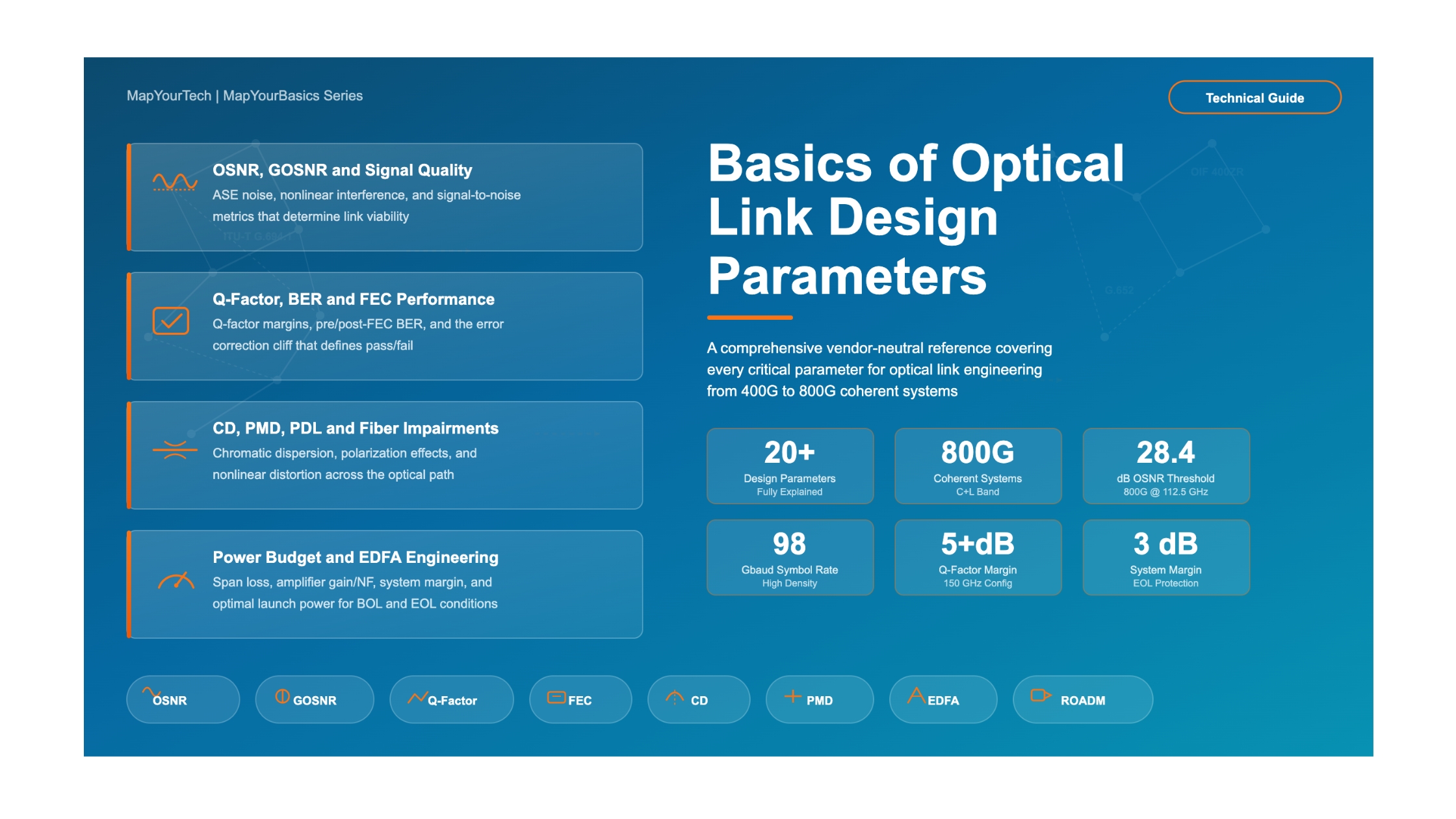

Basics of Important Parameters in DWDM Link Design
A comprehensive, vendor-neutral reference for optical network engineers covering every critical parameter in Dense Wavelength Division Multiplexing link engineering — from OSNR and chromatic dispersion to Q-factor margins and nonlinear impairments.
1. Introduction
Designing a Dense Wavelength Division Multiplexing (DWDM) optical link is not simply a matter of connecting two transceivers through fiber. It is an engineering exercise that demands careful balancing of dozens of interrelated parameters — each one capable of determining whether your link delivers error-free performance for 25 years or fails within weeks of commissioning. Every parameter tells a story about the physical health of the optical signal, and understanding that story is what separates successful deployments from troubled ones.
Optical link engineering has grown substantially more complex as the industry has moved from 10G direct-detect systems to 400G, 600G, and 800G coherent systems operating across both C-band and L-band. Modern coherent transceivers can compensate for many impairments electronically through Digital Signal Processing (DSP), but they still have hard limits. Exceeding those limits results in uncorrectable errors, service degradation, and — in the worst case — complete link failure. The parameters discussed in this article define exactly where those limits are and how much margin exists between your operating point and the failure threshold.
This article provides a complete, vendor-neutral reference for every critical parameter that appears in a typical DWDM link engineering report. For each parameter, we explain what it is, why it matters, how it is calculated, what values are acceptable, and what happens when it goes out of specification. The content is drawn from real-world link engineering data representing 800G coherent systems operating over 100 km G.652 fiber spans with inline amplification — a common deployment scenario in metro and regional networks.
2. The DWDM Link Engineering Framework
Before examining individual parameters, it is essential to understand the overall framework within which DWDM link engineering operates. Link engineering is the process of verifying that an optical signal can travel from a transmitter at Site A to a receiver at Site B (and vice versa) with sufficient quality to maintain error-free communication under all operating conditions — including fiber aging, component degradation, temperature variations, and repair splices accumulated over the system's lifetime.
2.1 Beginning of Life vs. End of Life
Every link engineering report evaluates two distinct scenarios. Beginning of Life (BOL) represents the system performance when fiber and components are brand new, with minimum loss and optimal conditions. End of Life (EOL) represents the worst-case scenario after years of operation, accounting for fiber degradation, additional splice losses from cable repairs, connector aging, and amplifier performance degradation. The difference between BOL and EOL performance directly determines how much margin the system has to absorb real-world impairments over its operational lifetime — typically 15 to 25 years.
Engineers design for EOL conditions because the system must work at its worst, not at its best. A link that works perfectly at BOL but fails at EOL has zero practical value. However, BOL performance must also be checked because excessively strong signals at the start of a link's life can cause nonlinear impairments that are equally destructive.
Figure 1: BOL vs. EOL performance degradation over system lifetime. The design must ensure EOL performance stays above the FEC threshold with adequate margin.
2.2 The Signal Path
A typical DWDM link consists of transmitter (transponder/muxponder), ROADM add/drop stage, pre-amplifier or booster EDFA, fiber span with connectors and splices, line amplifier (for longer spans), ROADM drop stage, and finally the receiver. Each element in this chain contributes loss, noise, and distortion. The link engineering process quantifies every contribution and verifies that the cumulative effect remains within the receiver's tolerance.
Figure 2: Signal path through a typical DWDM point-to-point link showing where different parameter categories originate.
3. Channel Configuration Parameters
Channel configuration parameters define the fundamental characteristics of each wavelength channel in the DWDM system. These parameters are set during network planning and directly determine the capacity, spectral efficiency, and reach of the optical link.
3.1 Operating Band (C-Band and L-Band)
DWDM systems operate within specific wavelength windows defined by the ITU-T. The C-band (Conventional band) covers approximately 1530 nm to 1565 nm, corresponding to frequencies around 191.4 THz to 196.0 THz. The L-band (Long band) extends from approximately 1565 nm to 1625 nm, covering frequencies from roughly 186.0 THz to 191.4 THz.
The choice of operating band affects multiple aspects of link design. C-band has lower fiber attenuation (around 0.20 dB/km for G.652 fiber) and is the traditional band for DWDM deployment with mature EDFA technology. L-band has slightly higher attenuation (around 0.22 dB/km) and different chromatic dispersion characteristics, but provides additional spectrum to effectively double system capacity when combined with C-band. The dispersion coefficient is higher in L-band — approximately 19.3 ps/(nm·km) at 1590 nm compared to about 16.7 ps/(nm·km) at 1550 nm in C-band.
What it tells the network owner: The operating band determines how many wavelengths the network can carry and directly scales the total system capacity. A C+L band system can carry roughly twice the channels of a C-band-only system, doubling potential revenue-generating capacity on the same fiber pair — though it requires investment in L-band amplifiers and C+L capable ROADMs.
3.2 Channel Frequency and Spacing
Each DWDM channel is assigned a specific center frequency from the ITU-T frequency grid (defined in ITU-T G.694.1). Common channel spacings include 50 GHz, 75 GHz, 100 GHz, 112.5 GHz, and 150 GHz. In modern flexible-grid systems, channel bandwidth can be assigned in increments of 12.5 GHz to optimize spectral utilization.
Channel spacing must be wider than the signal bandwidth to prevent inter-channel crosstalk. For example, an 800G signal using 98 Gbaud symbol rate with a channel bandwidth of 112.5 GHz leaves roughly 14.5 GHz of guard band. Tighter spacing improves spectral efficiency (more channels per fiber) but increases the risk of linear crosstalk and nonlinear inter-channel effects like Cross-Phase Modulation (XPM) and Four-Wave Mixing (FWM).
3.3 Number of Channels
The number of channels deployed on a fiber directly affects the total system capacity and the per-channel performance. More channels mean higher total optical power in the fiber, which increases nonlinear impairments. In link engineering, the system is typically designed for the maximum planned channel count (even if not all channels are deployed initially) to ensure performance remains acceptable at full capacity. Typical deployments range from 32 channels at 150 GHz spacing to 96 channels at 50 GHz spacing in C-band alone.
3.4 Line Rate, Symbol Rate, and Bits per Symbol
These three parameters are mathematically linked and together define the modulation configuration of each channel.
-- Fundamental relationship:

Line Rate = Symbol Rate × Bits per Symbol × Polarizations × Code Rate

Where:
  Line Rate        = Net data throughput (e.g., 800 Gb/s)
  Symbol Rate      = Baud rate of the modulated signal (e.g., 98 Gbaud)
  Bits per Symbol  = Constellation density (e.g., 4.21 for probabilistic shaping)
  Polarizations    = 2 (dual-polarization in coherent systems)
  Code Rate        = FEC overhead factor (typically 0.8 to 0.93)

-- Worked Example (800G at 112.5 GHz):
  Symbol Rate      = 98 Gbaud
  Bits per Symbol  = 4.21 (probabilistic shaping)
  Gross Rate       = 98 × 4.21 × 2 = ~825 Gb/s
  Net Data Rate    = ~800 Gb/s after FEC overhead

-- Worked Example (800G at 150 GHz):
  Symbol Rate      = 131.4 Gbaud
  Bits per Symbol  = 3.5
  Gross Rate       = 131.4 × 3.5 × 2 = ~920 Gb/s
  Net Data Rate    = ~800 Gb/s after FEC overhead
The symbol rate (measured in Gbaud) determines the occupied bandwidth of the signal. Higher symbol rates require wider channel spacing but allow lower-order modulation formats, which are more tolerant of noise. The bits per symbol value indicates the modulation format density — a value of 2 corresponds to QPSK, 3 to 8QAM, 4 to 16QAM, and fractional values indicate probabilistic constellation shaping (PCS), which is widely used in modern coherent systems to optimize capacity for a given reach.
What it tells the network owner: Higher bits per symbol means more data per channel but requires better OSNR. A system running 800G at 98 Gbaud with 4.21 bits/symbol needs about 28.4 dB OSNR — while the same 800G at 131.4 Gbaud with 3.5 bits/symbol needs only 26.9 dB OSNR. The lower-order modulation trades spectral efficiency for longer reach and higher noise tolerance.
| Line Rate | BW (GHz) | Symbol Rate (Gbaud) | Bits/Symbol | OSNR Threshold (dB) | Spectral Eff. (b/s/Hz) | Relative Reach |
|---|---|---|---|---|---|---|
| 400G | 75 | 63 | 3.97 | 19.8 | 5.33 | Longest |
| 400G | 112.5 | 98 | 2.55 | 17.9 | 3.56 | Very Long |
| 600G | 112.5 | 98 | 3.83 | 22.0 | 5.33 | Medium |
| 800G | 112.5 | 98 | 4.21 | 28.4 | 7.11 | Short-Medium |
| 800G | 150 | 131.4 | 3.50 | 26.9 | 5.33 | Medium-Long |
Table 1: Modulation format trade-offs for different line rate and bandwidth combinations.
4. Optical Signal-to-Noise Ratio (OSNR)
The Optical Signal-to-Noise Ratio (OSNR) is the single most important parameter in DWDM link engineering. It measures the ratio of signal power to Amplified Spontaneous Emission (ASE) noise power within a defined reference bandwidth (typically 0.1 nm or 12.5 GHz). OSNR is expressed in dB and directly determines whether the receiver can correctly decode the transmitted data.
4.1 OSNR Threshold
Every transceiver has a minimum OSNR requirement — the OSNR Threshold — below which the Forward Error Correction (FEC) engine cannot correct all errors, resulting in uncorrectable bit errors on the client interface. This threshold depends on the modulation format, FEC type, and implementation quality. For an 800G signal at 112.5 GHz bandwidth with 4.21 bits/symbol, a typical OSNR threshold is 28.4 dB. For a wider 150 GHz bandwidth at 3.5 bits/symbol carrying the same 800G, the threshold drops to 26.9 dB.
4.2 OSNR at EOL and BOL
The link engineering report provides OSNR values at both EOL and BOL operating conditions. The EOL OSNR is the critical value — it represents the worst-case noise performance after accounting for maximum fiber loss, worst-case amplifier noise figures, and all aging effects.
-- OSNR through a cascade of amplifiers:

  1/OSNR_total = Σ (1/OSNR_i)     (in linear, not dB)

Where each amplifier stage contributes:
  OSNR_i = 58 + P_in - NF_i    (dB, for 0.1 nm ref BW)

  P_in  = Input power to amplifier (dBm per channel)
  NF_i  = Noise Figure of amplifier (dB, typically 5-6 dB)

-- Worked Example (Single-span 100 km, C-Band):
  Tx OSNR          = 35.0 dB  (transceiver output)
  After Booster    = 32.5 dB  (EDFA adds ASE noise)
  After 100 km     = 32.5 dB  (fiber attenuates signal AND noise)
  After Pre-Amp    = 29.3 dB  (second EDFA adds more ASE)

  EOL OSNR at Rx   = 29.3 dB
  OSNR Threshold   = 28.4 dB
  OSNR Margin      = 29.3 - 28.4 = 0.9 dB
Engineering Guidance: A minimum OSNR margin of 1 dB above threshold is generally considered the absolute minimum for reliable operation. Most conservative designs target 2–3 dB of OSNR margin at EOL to account for measurement uncertainty, environmental variations, and unforeseen degradation.
4.3 Transmitter OSNR (Tx OSNR)
The transmitter OSNR represents the signal quality at the transceiver output before entering any network elements. Modern coherent transceivers typically produce a Tx OSNR of 35 dB or higher in-band (IB) and 38 dB or higher out-of-band (OOB). Tx OSNR is not infinite because the laser source and modulator introduce a small amount of noise. This parameter sets the upper bound on achievable link OSNR — no amount of amplification can improve the OSNR beyond what the transmitter produces.
Figure 3: OSNR Evolution Along the Signal Path
5. Generalized OSNR (GOSNR)
While traditional OSNR measures only the ratio of signal power to linear ASE noise, it does not account for nonlinear noise contributions. The Generalized OSNR (GOSNR) — sometimes called the effective OSNR — is a more comprehensive metric that includes both linear ASE noise and nonlinear interference noise (NLI) from fiber nonlinear effects.
-- GOSNR includes both ASE and nonlinear noise:

  1/GOSNR = 1/OSNR_ASE + 1/OSNR_NLI

Where:
  OSNR_ASE  = Traditional OSNR from amplifier ASE noise
  OSNR_NLI  = OSNR contribution from nonlinear interference

-- Worked Example:
  OSNR_ASE  = 29.3 dB
  OSNR_NLI  = 38.0 dB  (out-of-band OSNR contribution)

  1/GOSNR   = 1/851 + 1/6310 = 1.334e-3
  GOSNR     = 28.65 dB

  GOSNR is always lower than linear OSNR
  GOSNR Threshold = 27.4 dB
  GOSNR Margin    = 28.65 - 27.4 = 1.25 dB
GOSNR is always lower than or equal to the linear OSNR. The difference between the two indicates how much nonlinear penalty the system is experiencing. When OSNR and GOSNR values are close, the link is predominantly ASE-noise-limited. When the gap is large, nonlinear impairments are significant and launch power optimization becomes critical.
What it tells the network owner: GOSNR gives a more realistic picture of system performance than OSNR alone. If GOSNR is close to OSNR, the link has headroom for additional channels or higher launch powers. If GOSNR is much lower than OSNR, the link is approaching its nonlinear limit, and adding more channels or increasing power will degrade rather than improve performance.
6. Q-Factor, Q-Factor Margin, and BER
While OSNR measures signal quality in the optical domain, the Q-Factor and Bit Error Rate (BER) measure the actual digital signal quality at the DSP level. These parameters provide the definitive answer to whether the link works.
6.1 Q-Factor
The Q-factor is a dimensionless quality metric expressed in dB that represents the signal-to-noise ratio of the demodulated electrical signal. A higher Q-factor means better signal quality. The Q-factor is directly related to the BER through a mathematical function — for a Gaussian noise model, a Q-factor of 6 dB corresponds to a BER of approximately 1×10⁻⁹, though modern coherent systems with soft-decision FEC operate at much higher pre-FEC BER values.
6.2 Q-Factor Margin
The Q-Factor Margin is the difference between the calculated Q-factor and the minimum Q-factor required for the FEC to achieve error-free post-FEC operation. This is one of the most practical metrics in link engineering because it directly tells you how much additional degradation the system can tolerate before failing.
-- Q-Factor Margin:

  Q-Factor Margin = Q-Factor_measured - Q-Factor_FEC_limit

-- Example: 100 km, 800G C-Band, 112.5 GHz BW:

  Q-Factor EOL        = 5.997 dB
  Q-Factor BOL        = 6.604 dB
  FEC Limit Q-Factor  = 4.269 dB

  Q-Factor Margin EOL = 5.997 - 4.269 = 1.728 dB
  Q-Factor Margin BOL = 6.604 - 4.269 = 2.900 dB

-- Example: 100 km, 800G C-Band, 150 GHz BW:

  Q-Factor EOL        = 9.080 dB
  Q-Factor BOL        = 9.803 dB
  FEC Limit Q-Factor  = 4.074 dB

  Q-Factor Margin EOL = 9.080 - 4.074 = 5.006 dB
  Q-Factor Margin BOL = 9.803 - 4.074 = 6.145 dB
Notice the dramatic difference in Q-factor margin between the two configurations carrying the same 800G data rate. The 150 GHz configuration has over 5 dB of Q-factor margin at EOL compared to only 1.7 dB for the 112.5 GHz configuration. This illustrates the fundamental trade-off: wider channel spacing with lower-order modulation provides significantly more margin for the same distance, at the cost of using more spectrum per channel.
6.3 Pre-FEC BER and Post-FEC BER
The Pre-FEC BER represents the raw error rate before FEC correction. Modern soft-decision FEC codes can correct pre-FEC BER values up to 1.5×10⁻² to 2.4×10⁻² (1.5% to 2.4% of all bits). The Post-FEC BER is the residual error rate after correction. For telecom-grade service, the target is typically 10-15 or better — effectively error-free. When the report shows post-FEC BER of 0.0, the system has enough margin that the FEC produces zero residual errors.
Critical Point: If the pre-FEC BER exceeds the FEC threshold, the post-FEC BER rises above zero, and errors appear on the client interface. This is a hard cliff — there is no graceful degradation. The link either works with zero client errors, or it fails catastrophically with a flood of errors. This is why adequate margin in OSNR, GOSNR, and Q-factor is essential.
Figure 4: Q-Factor Margin Comparison — 112.5 GHz vs. 150 GHz at 800G
7. Optical Power Budget and Per-Channel Power
The optical power budget tracks the signal power level at every point in the link — from the transmitter output through every amplifier, ROADM, and fiber span to the receiver input. Maintaining the correct power level at every point is critical: too little power and the signal drowns in noise (poor OSNR); too much power and nonlinear effects corrupt the signal.
7.1 Transmitter Output Power
The transmitter (transponder) output power is the optical power launched into the network. Typical values for modern coherent transceivers range from -10 dBm to +4 dBm per channel, with a common default of -3.5 dBm to +2 dBm depending on the design. Some systems allow adjustable Tx power with user-configurable offsets to optimize the power budget for specific link conditions.
7.2 Per-Channel Power Through the Link
The link engineering report tracks the expected average, minimum, and maximum power per channel at every network element at both EOL and BOL. These values must stay within the acceptable operating range of each component.
| Network Element | Parameter | Avg Power EOL (dBm) | Avg Power BOL (dBm) | Function |
|---|---|---|---|---|
| Transponder Tx | Launch Power | -3.5 to +2.0 | -3.5 to +2.0 | Sets initial signal level |
| ROADM (Add) | After VOA/WSS | -15.5 to -11.2 | -15.5 to -11.2 | Attenuates to target per-ch power |
| Booster EDFA | Output | +5.2 to +7.0 | +5.4 to +7.0 | Amplifies to fiber launch power |
| Fiber Span (100 km) | After Span | -17 to -21 | -13 to -17 | Attenuated by fiber loss |
| Pre-Amp EDFA | Output | +5.2 to +5.7 | +5.0 to +5.6 | Recovers signal from span loss |
| ROADM (Drop) | After WSS | -2.3 to -2.8 | -2.3 to -2.8 | Drops to receiver |
| Receiver | Rx Power | -4.3 to -6.6 | -4.3 to -6.6 | Must be within Rx sensitivity |
Table 2: Per-channel power levels at each network element for a 100 km DWDM link.
7.3 Receiver Sensitivity and Dynamic Range
The receiver has a specific operating window defined by its sensitivity (minimum acceptable input power) and maximum input power. For noise-limited coherent receivers, typical sensitivity is around -14 dBm (for some configurations down to -18 dBm), while the maximum Rx power is typically +3 dBm. If received power falls below sensitivity, the signal-to-noise ratio is too poor for the DSP to lock. If it exceeds the maximum, the receiver photodetectors may saturate, causing distortion.
7.4 Span Loss and System Margin
-- Span Loss Calculation:

Total Span Loss = (Fiber Loss × Distance) + Splice Losses + Connector Losses + System Margin

-- Worked Example (100 km G.652, C-Band):
  Fiber attenuation = 0.20 dB/km × 100 = 20.0 dB
  Splice losses     = ~0.05 dB × 10    = 0.5 dB
  Connector losses  = 0.5 dB × 2      = 1.0 dB
  BOL Span Loss     = 20.0 + 0.5 + 1.0 = 21.5 dB
  System Margin     = 3.0 dB
  EOL Span Loss     = 21.5 + 3.0 = 24.5 dB

-- For L-Band (same fiber):
  Fiber attenuation = 0.22 dB/km × 100 = 22.0 dB
  EOL Span Loss     = 22.0 + 0.5 + 1.0 + 3.0 = 26.5 dB
The system margin (typically 3 dB for land-based networks) is a deliberate allocation for future fiber degradation. It represents the difference between the BOL and EOL calculations. Network owners should understand that this margin is consumed over time by cable repairs, environmental aging, and connector degradation — it is not “spare capacity” that can be reallocated.
7.5 EDFA Gain, Noise Figure, and Operating Mode
Erbium-Doped Fiber Amplifiers (EDFAs) are characterized by their gain (how much they amplify the signal, in dB) and noise figure (NF, how much ASE noise they add, in dB). A typical EDFA has a noise figure of 5–6 dB. The gain is set to compensate for the preceding span loss, so the amplifier output power equals the target launch power for the next span.
EDFAs can operate in different modes: Automatic Gain Control (AGC) maintains constant gain regardless of input power changes, which is the most common mode for line amplifiers. Automatic Power Control (APC) maintains constant output power. The choice of operating mode affects how the system responds to channel additions or removals and fiber cut events.
7.6 Total Power for All Channels
The total power is the aggregate optical power of all channels combined, and it is critical for staying within safe operating limits of fiber connectors, amplifiers, and laser safety regulations. For example, with 42 channels each at +5.5 dBm, the total power is approximately +21.7 dBm — a substantial amount that can exceed laser safety thresholds if not properly managed.
8. Fiber Impairment Parameters
As light travels through optical fiber, it encounters multiple physical effects that distort and degrade the signal. Modern coherent DSP can compensate for many of these impairments electronically, but each has a limit beyond which compensation is no longer effective.
8.1 Chromatic Dispersion (CD)
Chromatic Dispersion is the phenomenon where different wavelengths of light travel at slightly different speeds through the fiber. Since every optical signal occupies a finite bandwidth, the different spectral components arrive at the receiver at slightly different times, causing the signal pulses to broaden and overlap — a condition called Inter-Symbol Interference (ISI).
CD is measured in picoseconds per nanometer (ps/nm) and accumulates linearly with distance. For G.652 fiber, the dispersion coefficient is approximately 17 ps/(nm·km) at 1550 nm. Over 100 km, this produces approximately 1,677 ps/nm of accumulated dispersion in C-band and approximately 1,937 ps/nm in L-band (where the dispersion coefficient is higher).
-- Chromatic Dispersion Accumulation:

  CD_accumulated = D(λ) × L

Where:
  D(λ) = Dispersion coefficient at operating wavelength (ps/nm/km)
  L     = Fiber length (km)

-- Worked Examples:
  C-Band (1550 nm): D = 16.77 ps/nm/km
    CD = 16.77 × 100 = 1,677 ps/nm

  L-Band (1590 nm): D = 19.37 ps/nm/km
    CD = 19.37 × 100 = 1,937 ps/nm

-- Coherent DSP Compensation Range (typical):
  400G @ 112.5 GHz: ±70,000 ps/nm (~4,000 km G.652)
  800G @ 112.5 GHz: ±50,000 ps/nm (~3,000 km G.652)
  800G @ 150 GHz:   ±50,000 ps/nm (~3,000 km G.652)
Modern coherent DSP can compensate for enormous amounts of chromatic dispersion — often tens of thousands of ps/nm, corresponding to thousands of kilometers of fiber. This means CD is rarely a limiting factor in modern coherent systems on standard G.652 fiber. However, the DSP compensation range does have a finite limit, and exceeding it causes signal degradation. Additionally, higher-order modulation formats (more bits per symbol) are generally more sensitive to residual CD after DSP compensation.
What it tells the network owner: For metro and regional networks on G.652 fiber (up to ~1,000 km), chromatic dispersion is fully compensated by coherent DSP with no external compensation modules needed. This eliminates the cost and complexity of Dispersion Compensating Fiber (DCF) modules that were required in older 10G and 40G direct-detect systems. However, for ultra-long-haul submarine or terrestrial routes, CD accumulation must be carefully tracked to ensure it stays within the DSP’s compensation window.
8.2 Polarization Mode Dispersion (PMD)
Polarization Mode Dispersion is caused by slight asymmetries in the fiber core that make the two orthogonal polarization modes of light travel at slightly different speeds. Unlike CD, PMD is a statistical (random) process that accumulates as the square root of distance, not linearly. It is measured in picoseconds (ps) and is characterized by the fiber’s PMD coefficient in ps/√km.
-- PMD Accumulation (statistical):

  PMD_link = √( PMD_fiber² + PMD_component1² + PMD_component2² + ... )

-- Fiber PMD:
  PMD_fiber = PMD_coefficient × √L

-- Worked Example (100 km):
  Fiber PMD coefficient  = 0.1 ps/√km (modern G.652)
  Fiber PMD             = 0.1 × √100 = 1.0 ps

  Component contributions (RSS):
    Transponder         = 0 ps
    ROADM              = 0.5 ps
    EDFA #1            = 0.58 ps
    Fiber              = 0.99 ps
    EDFA #2            = 1.03 ps
    ROADM              = 1.15 ps
    Receiver           = 1.15 ps (total accumulated)

-- Typical PMD Tolerance:
  800G @ 98 Gbaud:  max ~30 ps
  800G @ 131 Gbaud: max ~30 ps
  400G @ 63 Gbaud:  max ~30 ps
Modern coherent DSP can compensate for substantial PMD — typically up to 30 ps for most transponder configurations. The 1.15 ps accumulated PMD in a 100 km link is far below this limit, providing enormous headroom. PMD becomes a concern primarily on older fiber plants with high PMD coefficients (>0.5 ps/√km) or on very long routes where the accumulated PMD approaches the DSP limit.
8.3 Polarization Dependent Loss (PDL)
Polarization Dependent Loss is the variation in insertion loss experienced by different polarization states passing through an optical component. Unlike PMD (which is a time-domain effect), PDL causes power imbalance between polarization states, which directly reduces the effective OSNR.
-- PDL Accumulation (statistical, RSS):

  PDL_total = √( PDL_1² + PDL_2² + PDL_3² + ... )

-- Worked Example (100 km link):
  ROADM       = 0.3 dB
  EDFA #1     = 0.5 dB
  Fiber       = 0.5 dB
  EDFA #2     = 0.64 dB
  ROADM       = 0.71 dB

  Total PDL   = 0.71 dB

-- PDL Tolerance (typical):
  Most transponders: max 2.0 dB
PDL is particularly insidious because it interacts with the polarization multiplexing used in coherent systems. Even a modest PDL of 1–2 dB can cause a noticeable OSNR penalty (0.5–1 dB), and this penalty varies randomly as the polarization state fluctuates. Each ROADM, amplifier, and connector adds to the accumulated PDL.
What it tells the network owner: PDL is one of the hardest impairments to manage because it accumulates through every passive and active component. Networks with many ROADM hops (mesh architectures with frequent add/drop) accumulate PDL faster and may need to limit the number of optical bypasses a wavelength traverses. Tight connector maintenance and using high-quality ROADM components with low PDL specifications directly improve network reliability.
8.4 Nonlinear Effects and Effective Accumulated Power
When optical power in the fiber exceeds a certain level, the fiber’s refractive index begins to change in proportion to the signal intensity, generating nonlinear impairments. The three main nonlinear effects in DWDM systems are Self-Phase Modulation (SPM), Cross-Phase Modulation (XPM), and Four-Wave Mixing (FWM). These effects corrupt the signal in ways that cannot be fully compensated by the DSP, and they represent the ultimate limit on how much data a fiber can carry.
The Effective Accumulated Power (also called accumulated nonlinear phase) quantifies the total nonlinear distortion the signal has experienced. It is measured in dB and depends on the launch power per channel, the number of channels, the fiber type (effective area and nonlinear coefficient), and the number of spans. Typical values for a single 100 km span range from 2 to 3.3 dB. Higher values indicate more nonlinear distortion.
Engineering Guidance: Nonlinear impairments set an upper bound on useful launch power. Increasing launch power beyond the optimal point degrades performance rather than improving it. The optimal launch power is the point where the total penalty (ASE noise + nonlinear noise) is minimized — this is often called the “nonlinear threshold” or the “sweet spot” in optical power optimization.
Figure 5: The nonlinear trade-off. Increasing launch power improves OSNR (left) but worsens nonlinear effects (right). The optimal launch power maximizes GOSNR.
9. Forward Error Correction (FEC) Parameters
Forward Error Correction is the mathematical coding scheme that adds redundant bits to the transmitted data, enabling the receiver to detect and correct errors without retransmission. FEC is what allows modern coherent systems to operate at pre-FEC BER levels of 1–2% while delivering error-free client data.
9.1 FEC Type and Overhead
Modern DWDM transceivers use either standard FEC (as defined by IEEE or OIF standards, such as KP4-FEC for 400ZR) or proprietary high-gain FEC (also called soft-decision or SD-FEC). Proprietary FEC codes typically provide 1–3 dB higher coding gain than standard FEC, which translates directly into longer reach or more margin. However, they require matching transceivers at both ends.
FEC overhead ranges from approximately 7% (hard-decision) to 25%+ (high-gain soft-decision). A 25% FEC overhead means that for every 100 bits of client data, 25 additional error-correction bits are transmitted. The trade-off is direct: higher FEC overhead means lower net throughput per symbol but higher tolerance for noise and impairments.
9.2 FEC Breach and Q0 Factor
The FEC Breach threshold is the pre-FEC BER level at which the FEC begins to fail. For typical proprietary SD-FEC, the FEC breach occurs at a pre-FEC BER around 2.0×10⁻² to 2.4×10⁻². The corresponding Q-factor at FEC breach is sometimes called Q0, and typical values range from 5.5 to 5.9 dB depending on the FEC implementation.
10. ROADM and Filtering Parameters
Reconfigurable Optical Add-Drop Multiplexers (ROADMs) enable wavelength-level routing without optical-electrical-optical conversion. Each ROADM passage introduces several impairments that accumulate across multi-hop paths.
10.1 ROADM Insertion Loss
Every ROADM passage introduces insertion loss — typically 8–12 dB per pass through the Wavelength Selective Switch (WSS). This loss must be compensated by adjacent amplifiers. In the data, ROADM attenuation values of -8 to -12 dB per passage are typical.
10.2 Filter Narrowing (Filter Concatenation)
Each ROADM WSS applies a bandpass filter to the signal. Multiple ROADM hops cause the effective filter bandwidth to narrow progressively. This filter concatenation effect clips the signal spectrum edges, causing inter-symbol interference and an effective OSNR penalty. The penalty increases with ROADM hops and is more severe for signals occupying a larger fraction of the channel bandwidth.
For signals using 98 Gbaud in a 112.5 GHz channel, the filter margin is relatively tight (~14.5 GHz each side). After 6–8 ROADM passes, the cumulative filter narrowing can introduce 0.5–2 dB penalty. For 131.4 Gbaud in 150 GHz, the margin is more comfortable (~18.6 GHz), allowing more ROADM hops.
What it tells the network owner: ROADM hop count is a critical design constraint. High-spectral-efficiency signals can traverse fewer ROADMs before filter narrowing degrades performance. This directly impacts network architecture decisions: mesh networks with many optical bypasses need wider channel spacing or lower baud rates than simple point-to-point links.
10.3 ROADM VOA Settings
The Variable Optical Attenuator (VOA) inside the ROADM equalizes per-channel power levels before they enter the multiplexer. This ensures all channels have approximately the same power at the booster EDFA input, which is essential for maintaining flat gain across all channels.
Figure 6: Parameter interaction map showing how input impairments flow through GOSNR to determine final link performance metrics.
11. Complete Parameter Reference Table
The following comprehensive table summarizes every parameter discussed in this article, with typical values, acceptable ranges, and practical significance.
| Parameter | Unit | Typical Range | Why It Matters | What Happens if Out of Spec |
|---|---|---|---|---|
| Operating Band | — | C-band / L-band / C+L | Determines total wavelength capacity | Wrong band = no signal; C+L doubles capacity |
| Channel Frequency | THz | 191.3–196.1 (C), 186–191.4 (L) | Assigns each channel to ITU grid slot | Frequency mismatch = channel collision or loss |
| Channel Spacing / BW | GHz | 50, 75, 100, 112.5, 150 | Determines channel count and spectral efficiency | Too tight = crosstalk; too wide = wasted spectrum |
| Number of Channels | — | 32–96 per band | Total system capacity; affects NL impairments | More channels = more NL; design for max count |
| Line Rate | Gb/s | 100, 200, 400, 600, 800 | Data capacity per wavelength | Higher rate = higher OSNR needed = shorter reach |
| Symbol Rate | Gbaud | 63–138 | Occupied bandwidth; affects CD/PMD tolerance | Higher baud = wider spectrum needed |
| Bits per Symbol | — | 2.0–5.6 | Modulation density; trade capacity vs. reach | Higher = more capacity but less noise tolerance |
| OSNR Threshold | dB | 17–28 (varies by config) | Minimum OSNR for FEC to correct all errors | Below threshold = uncorrectable errors |
| OSNR (EOL/BOL) | dB | 28–35 | Actual noise performance of the link | Below threshold + margin = link at risk |
| Tx OSNR | dB | 35 IB, 38 OOB | Upper bound on achievable OSNR | Low Tx OSNR degrades all downstream performance |
| GOSNR | dB | OSNR − 0.5 to 2 dB | OSNR including nonlinear noise — most realistic metric | Low GOSNR = system is NL-limited |
| GOSNR Threshold | dB | 1–2 dB below OSNR threshold | Minimum GOSNR for error-free operation | Below threshold = errors from NL+ASE combined |
| Q-Factor | dB | 5.5–12 | Electrical SNR after demodulation | Below FEC limit Q = errors on client interface |
| Q-Factor Margin | dB | 1.5–6+ (target ≥2) | Safety buffer above FEC cliff | <1 dB = risky; <0 dB = link failure |
| Pre-FEC BER | — | 10-3 to 2.4×10⁻² | Raw error rate before FEC correction | Above FEC limit = uncorrectable errors |
| Post-FEC BER | — | 0 (target <10-15) | Residual errors after FEC — the bottom line | >0 = errors reaching client equipment |
| Tx Power | dBm | -10 to +4 | Initial signal level into the network | Too low = poor OSNR; too high = NL effects |
| Rx Power | dBm | -18 to +3 | Must be within receiver dynamic range | Below sensitivity = no lock; above max = saturation |
| Span Loss | dB | 18–28 per 100 km | Total attenuation between amplifier sites | Exceeds EDFA gain = insufficient signal recovery |
| System Margin | dB | 3 (land), 1–2 (subsea) | Buffer for aging and repairs | Consumed over time; must be preserved |
| EDFA Gain | dB | 15–30 | Signal amplification; compensates span loss | Insufficient gain = OSNR degradation |
| EDFA Noise Figure | dB | 5–6 | ASE noise added per amplifier stage | Higher NF = lower OSNR = shorter reach |
| Chromatic Dispersion | ps/nm | 1,600–2,000 per 100 km | Pulse broadening; compensated by DSP | Exceeds DSP range = ISI and errors |
| PMD (accumulated) | ps | 0.5–5 (modern fiber) | Polarization-related pulse spreading | Exceeds DSP limit (~30 ps) = errors |
| PDL (accumulated) | dB | 0.3–2.0 | Polarization power imbalance; degrades OSNR | >2 dB = measurable OSNR penalty |
| Eff. Accumulated Power | dB | 2–4 per span | Nonlinear distortion strength | Higher = more NL impairment = GOSNR drop |
| FEC Type | — | Standard / Proprietary SD-FEC | Coding gain affects OSNR threshold | Wrong FEC = suboptimal threshold |
Table 3: Complete DWDM link design parameter reference with typical values and practical implications.
12. Practical Design Guidelines
Understanding individual parameters is essential, but successful DWDM link design requires managing their interactions. Here are practical guidelines for optical network engineers and network owners.
12.1 Margin Allocation Strategy
A well-designed DWDM link allocates margin across multiple categories. The total system margin is not a single number but a combination of individual allocations that protect against different degradation mechanisms.
| Margin Category | Typical Allocation (dB) | Purpose |
|---|---|---|
| Fiber aging and repairs | 3.0 | EOL vs. BOL span loss increase |
| EDFA gain flatness | 0.5–1.0 | Gain ripple across channels |
| Connector degradation | 0.5 | Cleaning, mating cycles |
| Temperature variation | 0.5–1.0 | Seasonal fiber property changes |
| Measurement uncertainty | 0.5 | OTDR and power meter accuracy |
| Unallocated contingency | 0.5–1.0 | Unknown unknowns |
| Total recommended | 5.5–7.0 | Comprehensive protection |
Table 4: Recommended margin allocation for a robust DWDM link design.
12.2 Design Verification Checklist
Before accepting a DWDM link engineering design, verify the following parameters meet their respective criteria:
Link Design Verification Checklist
- OSNR at EOL exceeds OSNR threshold by at least 1 dB (preferably 2–3 dB)
- GOSNR at EOL exceeds GOSNR threshold by at least 1 dB
- Q-factor margin at EOL is at least 1.5 dB (preferably 2+ dB)
- Post-FEC BER = 0 at both EOL and BOL conditions
- Rx power at EOL falls within receiver sensitivity and maximum input range
- Accumulated PMD is below 60% of transceiver PMD tolerance
- Accumulated PDL is below transceiver PDL tolerance (typically <2 dB)
- Accumulated chromatic dispersion is within DSP compensation range
- EDFA output power is within amplifier operating specification
- Total fiber launch power complies with laser safety requirements
- System margin of at least 3 dB is allocated for fiber aging
- Both directions (A→B and B→A) meet all criteria independently
12.3 Common Design Mistakes to Avoid
Designing only for BOL conditions. A link that works perfectly on day one but has no margin for fiber aging is a link that will fail within a few years. Always verify EOL performance first.
Ignoring nonlinear effects. Optimizing for maximum OSNR by increasing launch power past the nonlinear threshold actually degrades performance. GOSNR, not OSNR, should be the primary design metric.
Overlooking PDL accumulation. In networks with multiple ROADM hops, PDL can silently consume margin. Each ROADM adds 0.3–0.5 dB of PDL, and after 4–6 hops, the accumulated PDL becomes a significant contributor to OSNR penalty.
Using wrong channel count in design. Designing for 20 channels when 80 will eventually be deployed means the nonlinear penalties are underestimated by several dB. Always design for the maximum planned channel count from the beginning.
Assuming symmetric performance. The A→B and B→A directions often have different amplifier configurations, ROADM types, or fiber characteristics. Each direction must be independently verified.
Figure 6: Relative Impact of Key Parameters on Link Performance (dB penalty contribution)
13. Future Considerations
As the optical networking industry moves toward 1.6T and beyond per wavelength, the parameters discussed in this article remain fundamentally the same, but their relative importance shifts. Higher line rates demand higher OSNR (pushing toward 30+ dB thresholds), which shrinks margins and makes every fraction of a dB of penalty more consequential. Several trends are reshaping how these parameters are managed.
Wider bandwidth transceivers and S-band expansion. As C-band and L-band fill up, the industry is exploring the S-band (1460–1530 nm) for additional capacity. S-band has different fiber characteristics (higher attenuation, different dispersion profile) that require new amplifier technology (Thulium-doped fiber amplifiers, TDFA) and updated link engineering models.
Probabilistic constellation shaping becomes standard. PCS allows continuous tuning of bits per symbol (and therefore OSNR threshold) to exactly match available link margin. Rather than stepping between discrete modulation formats (QPSK, 8QAM, 16QAM), PCS transceivers can adjust in fine increments to extract maximum capacity from any given link.
Machine learning for real-time margin optimization. Traditional link engineering uses worst-case static calculations. Emerging approaches use real-time telemetry (actual OSNR, Q-factor, PMD, and NLI measurements) combined with ML models to dynamically adjust launch power, modulation format, and FEC parameters — reducing the need for conservative static margins.
Multi-band systems increase parameter complexity. C+L+S band systems triple the number of channels and introduce inter-band nonlinear effects (particularly Stimulated Raman Scattering, SRS) that shift power between bands. Link engineering tools must model these cross-band interactions to correctly predict per-channel performance.
14. Conclusion
DWDM link engineering is the disciplined practice of quantifying every source of signal degradation across the optical path and verifying that the receiver can still decode the data under worst-case conditions. The parameters covered in this article — OSNR, GOSNR, Q-factor, Q-factor margin, pre-FEC BER, post-FEC BER, chromatic dispersion, PMD, PDL, nonlinear effects, span loss, system margin, EDFA gain and noise figure, channel configuration, and ROADM filtering effects — form the complete toolkit for this verification.
For network owners, the most important takeaway is that these parameters are not abstract numbers on a report. Each one represents real physical phenomena that either enable or prevent revenue-generating services from operating reliably. A 2 dB Q-factor margin means your link can absorb two more fiber repair splices or one degraded amplifier before it fails. A 0.5 dB margin means one bad connector can take down the wavelength. Understanding these parameters and their acceptable ranges is essential for making informed decisions about network investment, capacity planning, and operational practices.
For design engineers, the message is equally clear: design conservatively for EOL conditions, use GOSNR rather than OSNR as the primary design metric, account for every component in the PDL and PMD budget, and always verify both directions independently. The cost of adequate margin at design time is far less than the cost of service outages during operation.
Summary
- OSNR and GOSNR are the primary signal quality metrics; GOSNR is more accurate as it includes nonlinear noise
- Q-factor margin is the most practical metric — it directly tells you how close the link is to failure
- Post-FEC BER is the bottom line: it must be zero for error-free service
- Chromatic dispersion and PMD are well-compensated by coherent DSP for metro/regional distances
- PDL and nonlinear effects are the hardest impairments to manage and often limit system performance
- System margin (3 dB typical) must be preserved for fiber aging — it is not spare capacity
- Both link directions (A→B and B→A) must be verified independently
References
- ITU-T Recommendation G.694.1 — Spectral grids for WDM applications: DWDM frequency grid.
- ITU-T Recommendation G.652 — Characteristics of a single-mode optical fibre and cable.
- ITU-T Recommendation G.698.2 — Amplified multichannel dense wavelength division multiplexing applications with single channel optical interfaces.
- ITU-T Recommendation G.697 — Optical monitoring for dense wavelength division multiplexing systems.
- OIF Implementation Agreement — 400ZR: 400G ZR coherent DWDM optical interface.
- IEEE 802.3ct — Physical Layers and Management Parameters for 400 Gb/s over DWDM Systems.
- Essiambre, R.-J. et al., “Capacity Limits of Optical Fiber Networks,” Journal of Lightwave Technology.
- Sanjay Yadav, “Optical Network Communications: An Engineer’s Perspective” — Bridge the Gap Between Theory and Practice in Optical Networking.
Developed by MapYourTech Team
For educational purposes in Optical Networking Communications Technologies
Note: This guide is based on industry standards, best practices, and real-world implementation experiences. Specific implementations may vary based on equipment vendors, network topology, and regulatory requirements. Always consult with qualified network engineers and follow vendor documentation for actual deployments.
Feedback Welcome: If you have any suggestions, corrections, or improvements to propose, please feel free to write to us at feedback@mapyourtech.com

Optical Communications & Network Automation Expert | Author of 3 Books for Optical Engineers | Founder, MapYourTech
Optical networking engineer with nearly two decades of experience across DWDM, OTN, coherent optics, submarine systems, and cloud infrastructure. Founder of MapYourTech. Read full bio →
Follow on LinkedIn