Introduction:

In the realm of optical communication, precision and reliability are paramount. Amidst the intricate components and techniques that ensure seamless data transmission, Differential Group Delay (DGD) emerges as a critical factor. This article takes you on a journey through the intricacies of DGD, unraveling its definition, implications, measurement techniques, and strategies for effective management. By the end, you’ll not only understand the concept of DGD but also appreciate its significance in maintaining the integrity of optical signals.

What is Differential Group Delay (DGD)?

Differential Group Delay (DGD) refers to the time difference between two orthogonal polarization states of an optical signal as it traverses a medium, such as a fiber-optic cable. This phenomenon arises due to various factors, including birefringence within the optical components and environmental conditions. DGD has the potential to degrade signal quality, leading to signal distortion, reduced data rates, and increased bit error rates.

The Role of DGD in Optical Communication:

DGD’s impact on optical communication is profound, influencing the overall system performance in multiple ways:

1. Signal Distortion:

DGD can cause pulse spreading and overlapping, leading to signal distortion and compromised data integrity.

2. Dispersion Compensation Challenges:

In high-speed optical systems, DGD poses challenges to dispersion compensation techniques, affecting data transmission over long distances.

3. Bit Error Rate (BER) Increase:

As DGD grows, the probability of bit errors occurring within the signal rises, directly impacting the reliability of the communication link.

4. System Robustness:

Managing DGD is crucial for ensuring the robustness of optical systems against external factors, such as temperature variations and mechanical stress.

Measuring Differential Group Delay: Techniques and Insights

Measuring DGD accurately is essential for identifying potential signal degradation and implementing effective mitigation strategies. Several techniques are employed for DGD measurement:

1. Interferometric Methods:

Interferometric techniques exploit interference between two orthogonal polarization states to determine DGD with high precision.

2. Time-Domain Methods:

Time-domain methods involve introducing a known time delay between polarization states and measuring the resultant phase difference.

3. Spectral Analysis:

Spectral analysis techniques utilize the spectral characteristics of the signal to calculate DGD based on phase variations.

Managing DGD: Strategies for Enhanced Signal Integrity

Efficiently managing DGD is imperative for maintaining optimal signal quality and system performance:

1. Polarization Mode Dispersion (PMD) Compensation:

Sophisticated PMD compensation techniques, such as adaptive compensation, can mitigate the effects of DGD.

2. Dispersion Compensation Modules:

Incorporating dispersion compensation modules helps counteract signal distortion caused by DGD.

3. Modulation Formats:

Selecting appropriate modulation formats can enhance the system’s tolerance to DGD-induced signal degradation.

4. Monitoring and Feedback:

Implementing real-time monitoring and feedback mechanisms enables dynamic adjustments to mitigate DGD-related issues.

Frequently Asked Questions about Differential Group Delay (DGD):

• Why does DGD occur in optical communication? DGD arises from the time delay difference between orthogonal polarization states caused by factors like fiber birefringence.
• How does DGD affect data transmission? DGD can lead to signal distortion, dispersion challenges, increased BER, and reduced system performance.
• What are the consequences of high DGD values? High DGD values can result in significant signal degradation, making reliable communication challenging.
• Can DGD be entirely eliminated? While complete elimination is challenging, effective mitigation strategies can minimize DGD’s impact on signal quality.

 Polarization mode dispersion (PMD) is a property of a single-mode fiber or an optical component where pulse spreading is caused by different propagation velocities of the signal’s two orthogonal polarizations. Optical fibers or optical components can be modeled with two orthogonal polarization axes called principal states of polarization (PSP). 

An optical signal propagating in a fiber is resolved into these two PSP axes. Each polarization axis (fast and slow axis) has a different propagation velocity. This is due to different refractive indexes in each axis caused by the birefringence of the material. The different velocities lead to pulse spreading at the receiver end.

PMD can be expressed as the square root of the fiber length multiplied by a proportionality coefficient. This coefficient is referred to as the PMD coefficient and is measured in units of picoseconds per square root kilometer (ps/√km). The PMD coefficient is typically specified by fiber cable manufacturers and represents the PMD characteristic for a particular length of that fiber.

Fiber characterization can be defined as the field measurement and recording of fiber span parameters that affect signal transmission over all or selected operating wavelengths. These measured parameters provide a true picture of the fiber span’s transmission limitations. They are used in network planning to ensure transmission links are designed within transceiver operating budgets and limits. Full fiber characterization is often necessary in modern high-speed link designs, where optical budgets are stretched to their maximum with little or no margin for error. Fiber quality can also be assessed with these parameters. Fiber characterization is performed after new fiber cable link construction, dark fiber purchase, or lease. This helps to ensure the fiber quality meets or exceeds required specifications and expectations. It also documents fiber parameters at the time of construction or acquisition for comparison with future measurements to determine fiber degradation due to aging, damage, and repair.

Macro bending: Macrobending is the attenuation associated with bending or wrapping the fiber. Light can “leak out” of a fiber when it is bent. As the bend becomes tighter, more light escapes. Macrobending loss, measured in decibels, increases at longer wavelengths where the optical confinement of the light is weaker. It also increases linearly with the number of turns. Traditionally, macrobending was not a limiting effect when cables were mostly of loose-tube or ribbon design and installed into ducts. The tightest bends incurred by fibers were in splice trays, where excess fiber would be stored in loops after jointing. This was reflected in the macrobending specification of ITU-T Recommendation G.652, where a minimum bend radius of 30 mm was defined to reflect typical splice tray dimensions and 100 turns were agreed upon to simulate the total excess fiber from all the splice sites between repeaters. But macrobending effects become more pronounced in networks installed close-to and within the building. Prevalent in this segment of the network are low-diameter mini-cables that are stripped-back designs, compared to the traditional sheathed loose-tube and ribbon cables. Lightweight and highly flexible, these new designs are preferred for their space efficiency (when installed into commensurately small micro-ducts) and ease of handling and routing (when installed on the inside and outside of buildings along tortuous paths). Bend radii of much less than 30 mm therefore have become commonplace.

Micro bending :Microbending attenuation of an optical fiber relates to the light signal loss associated with lateral stresses along the length of the fiber. The loss is due to the coupling from the fiber’s guided fundamental mode to lossy, higher-order radiation modes. Mode coupling occurs when fibers suffer small random bends along

the fiber axes. This random bending is usually caused by external mechanical stresses against the cable material that compress the fiber. The result is random, high-frequency perturbations to the fiber. Lateral stresses can be caused by pressure induced by manufacturing or installation or by temperature-induced dimensional changes in cabling materials that cause undesirable fiber/fiber or fiber/cable material interactions. These interactions can give rise to random microscopic bends or curvatures of <1-mm radius that create very small displacements of the fiber core from the fiber axis. Microbending effects can be seen at all the commonly used wavelengths in single mode fibers (1310, 1550, and 1625 nm), whereas macrobending effects are seen predominantly at 1550 and 1625 nm.

Latency is a time delay experienced in system and it describes how long it takes for data to get from transmission side to receiver side. In a fiber optical communication system, it is essentially the length of optical fiber divided by the speed of light in fiber core, supplemented with delay induced by optical and electro optical elements plus any extra processing time required by system, also called overhead. Signal processing delay can be reduced by using parallel processing based on large scale integration CMOS technologies.

Added to the latency due to propagation in the fiber, there are other path building blocks that affect the total data transport time. These elements include

•   opto-electrical conversion,
•   switching and routing,
•   signal regeneration,
•   Amplification,
•   chromatic dispersion (CD) compensation,
•   polarization mode dispersion (PMD) compensation,
•   data packing, digital signal processing (DSP),
•   protocols and addition forward error correction (FEC)

When the bit error occurs to the system, generally the OSNR at the transmit end is well and the fault is well hidden.

Decrease the optical power at the transmit end at that time. If the number of bit errors decreases at the transmit end, the problem is non-linear problem.

If the number of bit errors increases at the transmit end, the problem is the OSNR degrade problem.

One method to reduce FWM effects is to use transmission fiber that has high chromatic dispersion coefficient at the signal wavelength such as standard single-mode fiber SSMF (ITU-T G.652). The typical chromatic dispersion coefficient of SSMF is 18 ps/nm ⋅ km @ 1550 nm which helps to significantly reduce FWM from occurring. Even a lower chromatic dispersion coefficient significantly helps in reducing FWM such as NZ-DSF fiber (ITU-T G.655). This fiber is specially designed with low chromatic dispersion coefficient (~4 ps/nm ⋅ km @ 1550 nm) for extended transmission distance but high enough to significantly reduce FWM effects.

To reduce these effects is to lower signal power in the fiber or use fiber with a larger cross sectional area to reduce the signal power density.

A third method to help reduce FWM effects is to space signal channels unevenly. 

A fourth method to reduce FWM effects is to use DWDM systems with wide channel spacing. The magnitude of FWM effect is dependent on channel spacing. Wider spaced   

DWDM channels generate weaker FWM components.

Work of transmission systems is to transmit signal from one location to another location over media and receive signal error free. Lot of impairments caused by Transmission media, system components and by signal itself. As in DWDM network each channel which carries signals like SDH, SONET, and Ethernet propagates in optical domain it encounters with linear and nonlinear effects, which distort signal pulse shape and amplitude. As each signal generated and received by Transceivers or Transponders. When this distorted optical signal received by Transceiver, it converts the optical signal in electrical signal, which decodes the actual information like SDH, SONET or Ethernet carry over individual channel. In digital format the impact of optical Linear and nonlinear impairments are detected as BER. Because these impairments, changed the original patterns of pulse shape and amplitude of signal, pulse width expansion leads to inter symbol interference, and at receiver end this is decoded 1 as 0 or 0 as 1, which cause BER.

These nonlinear interactions can be divided into three main categories:

 (1) Brillouin effect,

(2) Kerr effect, and

(3) Raman effect.

Stimulated Brillouin Scattering (Brillouin effect)

Stimulated Brillouin scattering (SBS) is an inelastic phenomenon resulting from the scattering of photon inside the optical fiber. The scattered photon is slightly frequency downshifted compared to the initial photon, the energy difference being transferred to an acoustic phonon.

When increasing the launch power, the optical fiber practically acts as a mirror whose reflectance coefficient increases. As a result, the corresponding fiber loss can significantly grow and the induced reflections can degrade the system performance.

When low power is injected into the fiber, only intrinsic Rayleigh back-reflections occur and the level of reflections is very low (around 32 dB). When high power is launched in the fiber, the backscattered power increases because of the stimulated Brillouin scattering

The SBS-related penalty can be minimized by keeping the per-channel power below the SBS threshold, which depends on the size of the optical fiber core and on the transmitter linewidth

Kerr Effect

In the case of a single-channel transmission, the refractive index of the waveguide is modulated by the fluctuations of the channel intensity via the Kerr effect. The amplitude of this phenomenon is increased by a high launch power and small effective area inside the optical fiber. This nonlinear effect can broaden the channel spectrum and therefore interplay with the chromatic dispersion, resulting in pulse distortion and broadening.

The Kerr effect is usually decomposed in three different contributions that are actually closely related. When a signal travels alone through the fiber, its modulated power induces a self-phase modulation (SPM). By contrast, the presence of several channels in a WDM transmission generates on each signal a cross-phase modulation. For the particular case of well-phase-matched WDM signals (i.e. moderate fiber chromatic dispersion), the Kerr effect produces four- wave mixing (FWM).

                 1. Self-Phase Modulation 

Light travels more slowly when the optical power is high, leading to a phase difference compared to light traveling at a low optical power. The result of the propagation of an amplitude-modulated signal is known as SPM.Self-phase modulation becomes significant as soon as the launch power is typically larger than 12 dBm.

                 2. Cross-Phase Modulation 

In the case of several high-power channels propagating simultaneously within the same fiber, the refractive index modulation experienced by one given channel is not only caused by the intensity modulation of this specific channel (SPM) but also by the intensity modulation brought by the copropagating channels. This cross-refractive index modulation is called cross-phase modulation (XPM) and can be described as a process through which the intensity fluctuations in a particular channel are converted to phase fluctuations in the other channels.

                 3. Four-Wave Mixing 

When several carriers at different wavelengths are launched into the fiber and are closed to be phase-matched, new waves can be generated by four-wave mixing via third-order intermodulation process. The optical frequencies of these FWM-generated waves are given by nijk= ni

+ nj -nk where ni ; nj , and nk are the frequencies of the launched initial channels (i.e., the signal channels). Four-wave mixing can transfer a fraction of the channel powers to the frequency of the other channels through the generation of FWM waves. FWM is considered the most dominant source of crosstalk in WDM systems .It becomes a major source of nonlinear crosstalk when- ever the channel spacing and fiber dispersion are small enough to satisfy the phase- matching condition approximately. For an N-channel system, i, j , and k can vary from 1 to N, resulting in a large combination of new frequencies generated by FWM. In the case of equally spaced channels, the new frequencies coincide with the existing frequencies, leading to coherent in-band crosstalk. When channels are not equally spaced, most FWM components fall in between the channels and lead to incoherent out-of-band crosstalk. In both cases, system performance is degraded because power transferred to each chan- nel through FWM acts as a noise source, but the coherent crosstalk degrades system performance much more severely.

Stimulated Raman Scattering 

Like SBS, stimulated Raman scattering (SRS) is an inelastic phenomenon resulting from the scattering of an incoming photon inside the optical fiber. The scattered photon is frequency downshifted compared to the initial photon, the energy difference being transferred to an optical phonon. When several beams propagate through the fiber at different wavelengths, the maximum energy transfer occurs for a 13.2-THz separation between the channels .

Channel interaction due to Raman scattering is not maximal for channel spacing lower than 13.2 THz, which is the case for WDM systems; nevertheless, it can still be significant for high-power, wideband systems.

Nonlinear effects are the impairments in optical signal caused by interaction of power levels of various signals in fiber. Non-linear interactions between the signal and the silica fiber transmission medium begin to appear as optical signal powers are increased to achieve longer span lengths at high bit rates. Consequently, non-linear fiber behavior has emerged as an important consideration both in high capacity systems and in long unregenerated routes.

 A variety of parameters influence the severity of these non-linear effects, including line code (modulation format), transmission rate, fiber dispersion characteristics, the effective area and non-linear refractive index of the fiber, the number and spacing of channels in multiple channel systems, overall unregenerated system length, as well as signal intensity and source line-width.

Each data channel in a DWDM link is a train of pulses. Being finite in time, each optical pulse is composed of a range of wavelengths distributed around a central optical wavelength, which corresponds to the central wavelength of a specific DWDM channel. The total signal in the optical fiber is then the combination of all the DWDM optical channels multiplexed in the optical fiber. During propagation in the optical fiber, the shape and amplitude of each pulse is modified by various effects arising from the physical properties of the optical fiber material.

Linear Impairments: Impairments increases linearly as signal propagates in fiber with distance known as linear impairments like attenuation and dispersion.

Counter pump distributed Raman amplifiers are often combined with EDFA pre-amps to extend span distances. This hybrid configuration can provide 6 dB improvement in the OSNR, which can significantly extend span lengths or increase span loss budget. Counter pump Raman Amplifier can also help reduce nonlinear effects by allowing for channel launch power reduction.

Raman Amplifiers are very sensitive to input power so they are always used with EDFA in cascaded fashion. (a small change at input will result in high output power change and thus subsequent components may suffer)

Forward pumping provides the highest SNR, and the smallest noise figure, because most of the Raman gain is then concentrated toward the input end of the fiber where power levels are high. However, backward pumping is often employed in practice because of other considerations such as the transfer of pump noise to signal and the effects of residual fiber birefringence. 

Major Noise sources of Raman Amplifiers are:

• Amplified spontaneous emissions (ASE)
• Double Rayleigh scattering (DRS)
• Pump laser noise.

ASE noise is due to photon generation by spontaneous Raman scattering.DRS noise occurs when twice reflected signal power due to Rayleigh scattering is amplified and interferes with the original signal as crosstalk noise. The strongest reflections occur from connectors and bad splices. Typically, DRS noise is less than ASE noise, but for multiple Raman spans it can add up. To reduce this interference, ultra-polish connectors (UPC) or angle polish (APC) connectors can be used. Optical isolators can be installed after the laser diodes to reduce reflections into the laser. Also span OTDR traces can help locate high-reflective events for repair.

Counter pump DRA configuration results in better OSNR performance for signal gains of 15 dB and greater. Pump laser noise is less of a concern because it usually is quite low with RIN of better than 160 dB/Hz.

Nonlinear Kerr effects can also contribute to noise due to the high laser pump power. For fibers with low DRS noise, the Raman noise figure due to ASE is much better than the EDFA noise figure. Typically, the Raman noise figure is –2 to 0 dB, which is about 6 dB better than the EDFA noise figure.

Raman amplifier noise factor is defined as the OSNR at the input of the amplifier to the OSNR at the output of the amplifier.

An undesirable feature is that the Raman gain is somewhat polarization sensitive. In general, the gain is maximum when the signal and pump are polarized along the same direction but is reduced when they are orthogonally polarized.

Advantages of Raman Amplifiers

1. 1. Signal Amplification Efficiency: Raman amplifiers utilize the Raman scattering phenomenon to amplify optical signals. This process enables efficient signal amplification across a broad range of wavelengths, facilitating multi-channel transmission.
   2. Wavelength Versatility: Unlike traditional amplifiers that work within specific wavelength ranges, Raman amplifiers can amplify signals at various wavelengths simultaneously. This versatility is particularly beneficial in dense wavelength division multiplexing (DWDM) systems.
   3. Extended Transmission Distance: Raman amplification effectively mitigates signal loss over long distances. By continuously boosting signals along the transmission path, Raman amplifiers enable high-quality communication links spanning thousands of kilometers.
   4. Reduced Nonlinear Effects: Raman amplification reduces the impact of nonlinear effects that can degrade signal quality in long-haul communication. This advantage contributes to maintaining the integrity of the transmitted data.
   5. Wide Bandwidth Coverage: The inherent characteristics of Raman amplifiers provide a wider bandwidth coverage, allowing them to support high-capacity data transmission, including high-definition video streaming and data-intensive applications.
   6. Enhanced Network Flexibility: Raman amplifiers offer flexibility in designing and optimizing optical networks. Network architects can adapt the system to accommodate changes in traffic demands and new services more effectively.
   7. Lower Noise Contribution: Raman amplification generates less amplified spontaneous emission (ASE) noise compared to other amplification methods. This results in improved signal-to-noise ratios, enhancing the overall quality of data transmission.
   8. Minimal Dispersion Impact: Raman amplifiers have a reduced impact on dispersion, which is the spreading of optical pulses as they travel through the fiber. This advantage translates to enhanced data integrity and reduced need for dispersion compensation.
   9. Energy Efficiency: Raman amplifiers consume less power compared to other types of amplifiers, contributing to more energy-efficient optical networks.
   10. Compatibility with Other Amplifiers: Raman amplifiers can be integrated seamlessly with other amplifier types, such as erbium-doped fiber amplifiers (EDFAs), to create hybrid systems that optimize performance.

Raman amplifier is a well-known amplifier configuration. This amplifier uses conventional fiber (rather doped fibers), which may be co-or counter-pumped to provide amplification over a wavelength range which is a function of the pump wavelength. The Raman amplifier relies upon forward or backward stimulated Raman scattering. Typically, the pump source is selected to have a wavelength of around 100 nm below the wavelength over which amplification is required.

Principle of working:

As the pump laser photons propagate in the fiber, they collide and are absorbed by fiber molecules or atoms. This excites the molecules or atoms to higher energy levels. The higher energy levels are not stable states so they quickly decay to lower intermediate energy levels releasing energy as photons in any direction at lower frequencies. This is known as spontaneous Raman scattering or Stokes scattering and contributes to noise in the fiber.

Since the molecules decay to an intermediate energy vibration level, the change in energy is less than the initial received energy during molecule excitation. This change in energy from excited level to intermediate level determines the photon frequency since Δ f = Δ E / h. This is referred to as the Stokes frequency shift and determines the Raman gain versus frequency curve shape and location. The remaining energy from the intermediate level to ground level is dissipated as molecular vibrations (phonons) in the fiber. Since there exists a wide range of higher energy levels, the gain curve has a broad spectral width of approximately 30 THz.

During stimulated Raman scattering, signal photons co-propagate frequency gain curve spectrum, and acquire energy from the Stokes wave, resulting in signal amplification.

Some of the information bullet to know is:

• The Raman amplifier is typically much more costly and has less gain than an Erbium Doped Fiber Amplifier (EDFA) amplifier. Therefore, it is used only for specialty applications.
• The main advantage that this amplifier has over the EDFA is that it generates very less noise and hence does not degrade span Optical to Signal Noise Ratio (OSNR) as much as the EDFA.
• Its typical application is in EDFA spans where additional gain is required but the OSNR limit has been reached.
• Adding a Raman amplifier might not significantly affect OSNR, but can provide up to a 20dB signal gain.
• Another key attribute is the potential to amplify any fiber band, not just the C band as is the case for the EDFA. This allows for Raman amplifiers to boost signals in O, E, and S bands (for Coarse Wavelength Division Multiplexing (CWDM) amplification application).
• The amplifier works on the principle of Stimulated Raman Scattering (SRS), which is a nonlinear effect.
• It consists of a high-power pump laser and fiber coupler (optical circulator).
• The amplification medium is the span fiber in a Distributed Type Raman Amplifier (DRA).
• Raman amplifiers can work at any wavelength as long as the pump wavelength is suitably chosen. It can work in C and L bands.
• Distributed Feedback (DFB) laser is a narrow spectral bandwidth which is used as a safety mechanism for Raman Card. DFB sends pulse to check any back reflection that exists in the length of fiber. If no High Back Reflection (HBR) is found, Raman starts to transmit.
• Generally, HBR is checked in initial few kilometers of fibers to first 20 Km. If HBR is detected, Raman will not work. Some fiber activity is needed after you find the problem area via OTDR.

DWDM (Dense Wavelength Division Multiplexing) technology is widely used to increase the capacity of optical networks. Amplifiers play a crucial role in boosting the signal strength and ensuring reliable transmission over long distances. However, the quality of amplifier performance can be affected by several factors, including gain tilt and gain ripple. In this article, we will explore what gain tilt and gain ripple are, how they impact the performance of DWDM amplifier links, and how to mitigate their effects.

Table of Contents

1. Introduction
2. Understanding DWDM Amplifier Links
3. What is Gain Tilt?
4. Causes of Gain Tilt
5. Effects of Gain Tilt
6. What is Gain Ripple?
7. Causes of Gain Ripple
8. Effects of Gain Ripple
9. How to Measure Gain Tilt and Gain Ripple
10. Mitigation Techniques for Gain Tilt and Gain Ripple
11. Conclusion
12. FAQs

1. Introduction

DWDM technology is widely used to increase the capacity of optical networks. Amplifiers play a crucial role in boosting the signal strength and ensuring reliable transmission over long distances. However, the quality of amplifier performance can be affected by several factors, including gain tilt and gain ripple. In this article, we will explore what gain tilt and gain ripple are, how they impact the performance of DWDM amplifier links, and how to mitigate their effects.

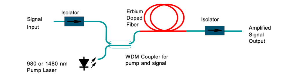
2. Understanding DWDM Amplifier Links

DWDM amplifier links consist of several optical amplifiers connected in series to compensate for the signal loss over long distances. The optical signal is amplified in each amplifier, and the output of the previous amplifier becomes the input for the next amplifier. The amplifiers are designed to provide a constant gain over a wide range of wavelengths to compensate for the loss due to dispersion, attenuation, and other factors. However, the gain of the amplifier may not be perfectly flat, and this can lead to gain tilt and gain ripple.The ability to control and adjust per channel optical power equalization is a principal feature of Amplifier in network applications. A major parameter to assure optical spectrum equalization throughout the DWDM system is the gain flatness of erbium-doped fiber amplifiers (EDFAs).

3. What is Gain Tilt?

Gain tilt is a phenomenon where the gain of the amplifier varies with the wavelength. In other words, the gain is not constant across the entire wavelength range, and there is a gradual increase or decrease in the gain as the wavelength changes. This can result in a distortion of the optical signal, especially if the signal contains multiple wavelengths.

4. Causes of Gain Tilt

The most common cause of gain tilt in DWDM amplifier links is the variation in the gain of the individual amplifiers. The gain of the amplifier depends on several factors, including the doping concentration, the pump power, the fiber length, and the temperature. Any variation in these factors can result in a variation in the gain, leading to gain tilt.

5. Effects of Gain Tilt

The effects of gain tilt can be severe, especially if the signal contains multiple wavelengths. The gain tilt can result in a distortion of the signal, causing errors and impairments in the transmission. The distortion can be mitigated by equalizing the gain across all wavelengths, which can be achieved using various techniques.

6. What is Gain Ripple?

Gain ripple is a phenomenon where the gain of the amplifier varies periodically with the wavelength. In other words, the gain is not constant, and there are peaks and dips in the gain as the wavelength changes. This can result in a distortion of the optical signal, especially if the signal contains multiple wavelengths.

7. Causes of Gain Ripple

The most common cause of gain ripple in DWDM amplifier links is the interference between the optical signals and the amplifiers. The interference can be caused by several factors, including the reflection from the fiber ends, the Rayleigh scattering, and

the amplifier noise. The interference can cause some wavelengths to be amplified more than others, resulting in the periodic gain variation, or gain ripple.

8. Effects of Gain Ripple

The effects of gain ripple can be severe, especially if the signal contains multiple wavelengths. The gain ripple can result in a distortion of the signal, causing errors and impairments in the transmission. The distortion can be mitigated by equalizing the gain across all wavelengths, which can be achieved using various techniques.

9. How to Measure Gain Tilt and Gain Ripple

The gain tilt and gain ripple can be measured using a specialized device called an optical spectrum analyzer (OSA). The OSA measures the power and the spectrum of the optical signal and provides a graphical representation of the gain tilt and gain ripple. The OSA can be used to identify the location and the magnitude of the gain tilt and gain ripple and help in the troubleshooting and optimization of the amplifier links.

10. Mitigation Techniques for Gain Tilt and Gain Ripple

The gain tilt and gain ripple can be mitigated using several techniques, including:

10.1. Pre-Equalization

Pre-equalization is a technique where the gain of the amplifiers is adjusted before the signal is transmitted. The adjustment compensates for the gain tilt and gain ripple and ensures that the signal is transmitted with a constant gain across all wavelengths. Pre-equalization can be performed using various devices, including the optical equalizer and the dynamic gain equalizer.

10.2. Post-Equalization

Post-equalization is a technique where the gain of the amplifiers is adjusted after the signal is transmitted. The adjustment compensates for the gain tilt and gain ripple and ensures that the signal is received with a constant gain across all wavelengths. Post-equalization can be performed using various devices, including the optical equalizer and the dynamic gain equalizer.

10.3. Optical Filters

Optical filters are devices that selectively transmit or reflect certain wavelengths of light. Optical filters can be used to equalize the gain across all wavelengths by selectively transmitting or reflecting the wavelengths that are affected by the gain tilt and gain ripple.

11. Conclusion

Gain tilt and gain ripple are common phenomena that can affect the performance of DWDM amplifier links. The gain tilt and gain ripple can cause distortion of the optical signal, resulting in errors and impairments in the transmission. The gain tilt and gain ripple can be mitigated using various techniques, including pre-equalization, post-equalization, and optical filters. The measurement and optimization of the gain tilt and gain ripple can be performed using an optical spectrum analyzer. By addressing the gain tilt and gain ripple, the performance of the DWDM amplifier links can be improved, and the reliability and efficiency of the optical networks can be enhanced.

12. FAQs

1. What is DWDM technology? DWDM (Dense Wavelength Division Multiplexing) is a technology used to increase the capacity of optical networks by transmitting multiple wavelengths of light over a single fiber.
2. What is an optical amplifier? An optical amplifier is a device that amplifies the optical signal without converting it to an electrical signal.
3. How does gain tilt affect the optical signal? Gain tilt can cause distortion of the optical signal, resulting in errors and impairments in the transmission.
4. What is an optical spectrum analyzer? An optical spectrum analyzer (OSA) is a device that measures the power and spectrum of the optical signal and provides a graphical representation of the gain tilt and gain ripple.
5. How can gain tilt and gain ripple be mitigated? Gain tilt and gain ripple can be mitigated using various techniques, including pre-equalization, post-equalization, and optical filters. These techniques can equalize the gain across all wavelengths, ensuring a constant gain and reducing the distortion of the optical signal.
   6. What are the causes of gain ripple? The most common cause of gain ripple is the interference between the optical signals and the amplifiers. The interference can be caused by several factors, including the reflection from the fiber ends, the Rayleigh scattering, and the amplifier noise.
   7. How can the gain tilt and gain ripple be measured? The gain tilt and gain ripple can be measured using an optical spectrum analyzer (OSA), which measures the power and spectrum of the optical signal and provides a graphical representation of the gain tilt and gain ripple.
   8. What are the benefits of addressing the gain tilt and gain ripple? By addressing the gain tilt and gain ripple, the performance of the DWDM amplifier links can be improved, and the reliability and efficiency of the optical networks can be enhanced. This can lead to increased capacity, better quality of service, and reduced downtime.
   9. What is pre-equalization? Pre-equalization is a technique where the gain of the amplifiers is adjusted before the signal is transmitted. The adjustment compensates for the gain tilt and gain ripple and ensures that the signal is transmitted with a constant gain across all wavelengths.
   10. What is post-equalization? Post-equalization is a technique where the gain of the amplifiers is adjusted after the signal is transmitted. The adjustment compensates for the gain tilt and gain ripple and ensures that the signal is received with a constant gain across all wavelengths.

Optical amplifiers are essential components in optical communication systems. They are used to amplify the optical signals transmitted over long distances. The performance of optical amplifiers is critical in ensuring the quality of the communication system. There are two modes of operation for optical amplifiers: power control mode and gain control mode. In this article, we will discuss the difference between these two modes and their applications. We will also provide some examples of optical amplifiers that use these modes.

Table of Contents

• Introduction
• What is Power Control Mode in Optical Amplifiers?
• Advantages of Power Control Mode
• Disadvantages of Power Control Mode
• Examples of Optical Amplifiers that Use Power Control Mode
• What is Gain Control Mode in Optical Amplifiers?
• Advantages of Gain Control Mode
• Disadvantages of Gain Control Mode
• Examples of Optical Amplifiers that Use Gain Control Mode
• Comparison between Power Control Mode and Gain Control Mode
• Conclusion
• FAQs

What is Power Control Mode in Optical Amplifiers?

Power control mode in optical amplifiers is a method of controlling the output power of the amplifier. In this mode, the output power of the amplifier is kept constant by adjusting the input power. This is achieved by using a feedback loop that measures the output power and adjusts the input power accordingly. Power control mode is commonly used in erbium-doped fiber amplifiers (EDFAs) and semiconductor optical amplifiers (SOAs).

Advantages of Power Control Mode

One of the advantages of power control mode is that it provides a stable output power. This is important in optical communication systems where the quality of the signal is critical. Another advantage is that it allows for a larger dynamic range of operation. This means that the amplifier can handle a wider range of input power levels without saturating or clipping.

Disadvantages of Power Control Mode

One of the main disadvantages of power control mode is that it is susceptible to fluctuations in the input power. This can result in changes in the output power, which can affect the quality of the signal. Another disadvantage is that it requires a feedback loop, which adds complexity to the amplifier.

Examples of Optical Amplifiers that Use Power Control Mode

Some examples of optical amplifiers that use power control mode are:

• Erbium-doped fiber amplifiers (EDFAs)
• Semiconductor optical amplifiers (SOAs)
• Raman amplifiers

What is Gain Control Mode in Optical Amplifiers?

Gain control mode in optical amplifiers is a method of controlling the gain of the amplifier. In this mode, the gain of the amplifier is kept constant by adjusting the pump power. This is achieved by using a feedback loop that measures the output power and adjusts the pump power accordingly. Gain control mode is commonly used in optical amplifiers that have a high gain, such as rare-earth-doped fiber amplifiers (REDFAs).

Advantages of Gain Control Mode

One of the advantages of gain control mode is that it provides a stable gain. This is important in optical communication systems where the quality of the signal is critical. Another advantage is that it is less susceptible to fluctuations in the input power. This is because the pump power is adjusted to maintain a constant gain, regardless of changes in the input power.

Disadvantages of Gain Control Mode

One of the main disadvantages of gain control mode is that it requires a high pump power. This can result in increased power consumption and higher operating costs. Another disadvantage is that it is less flexible than power control mode. This is because the gain is kept constant, which limits the dynamic range of operation.

Examples of Optical Amplifiers that Use Gain Control Mode

Some examples of optical amplifiers that use gain control mode are:

• Rare-earth-doped fiber amplifiers (REDFAs)
• Distributed Raman amplifiers (DRAs)
• Hybrid amplifiers

Comparison between Power Control Mode and Gain Control Mode

Both power control mode and gain control mode have their advantages and disadvantages. The choice of mode depends on the requirements of the application. Power control mode is suitable for applications where a stable output power is required, and a large dynamic range of operation is needed. Gain control mode, on the other hand, is suitable for applications where a stable gain is required, and high pump power is available.

Conclusion

Optical amplifiers are crucial components in optical communication systems. Power control mode and gain control mode are two modes of operation for optical amplifiers that are commonly used. Power control mode provides a stable output power and a large dynamic range of operation. Gain control mode provides a stable gain and is less susceptible to fluctuations in the input power. The choice of mode depends on the requirements of the application.

FAQs

1. What is an optical amplifier?
   • An optical amplifier is a device that amplifies the optical signal transmitted over long distances in optical communication systems.
2. What is power control mode?
   • Power control mode is a method of controlling the output power of the amplifier by adjusting the input power.
3. What is gain control mode?
   • Gain control mode is a method of controlling the gain of the amplifier by adjusting the pump power.
4. Which mode is better, power control or gain control?
   • The choice of mode depends on the requirements of the application. Power control mode is suitable for applications where a stable output power is required, and a large dynamic range of operation is needed. Gain control mode is suitable for applications where a stable gain is required, and high pump power is available.
5. What are some examples of optical amplifiers that use power control mode?
   • Some examples of optical amplifiers that use power control mode are EDFAs, SOAs, and Raman amplifiers.

Based on  placements, for a DWDM link there are three types of amplifiers:

• Booster Amplifier
• Pre-Amplifier
• In-Line Amplifier

Booster Amplifier 

Main purpose of booster amplifier is to boost the power transmitted.

 A booster amplifier is used to amplify the signal channels exiting the transmitter to the level required for launching into the fiber link. In most applications this level is in the range of 0-5 dBm per channel, however, it can be higher for more demanding applications. A booster is not always required in single channel links, but is essential in a WDM link where the multiplexer attenuates the signal channels. A booster amplifier typically has low gain (in the range of 5-15 dB) and high output power, typically about 20dBm for a 40 channel WDM system. The NF of a booster amplifier is not usually a critical parameter. At the other end of a link a pre-amplifier may be required to amplify the optical signal to the level where it can be detected over and above the thermal noise of the receiver.

Pre-Amplifier

These amplifiers are commonly used to improve the receiver sensitivity. Transmission distance can also be increased by putting an amplifier just before the receiver to boost the received power.

A pre-amplifier should provide high gain, often in the range of 30 dB, and have a low NF in the range of 4-5.5 dB, in order to assure error-free detection of the signal channels. The output power of the pre-amplifier need not be very high.

For links up to about 150 km, a booster and/or pre-amplifier are usually sufficient to ensure error-free transmission. However, for links above 150 km the performance deteriorates to such an extent that the signal becomes undetectable.

In-Line Amplifier

These amplifiers are used for compensating distribution losses in local-area networks. replace electronic regenerators. An in-line amplifier is characterized by large gain and low noise to amplify an already attenuated signal so that it can travel an additional length of fiber.

In-line amplifiers are placed every 80-100 km to ensure that the optical signal level remains above the noise floor. In-line amplifiers typically require moderate gain in the range of 15-25 dB, and NF in the range of 5-7 dB. Output power requirements are similar to those of booster amplifiers. While in the early days of optical amplifiers different amplifier models had to be specifically tailored for each of the above functions, today the technology has advanced so that a single well designed amplifier model can perform many of the functions for typical applications. However, there still remain challenging applications which require specially designed amplifiers, such as very high output power boosters, or ultra-low noise pre-amplifiers.

Advantages and drawbacks of EDFAs are as follows:-

Advantages:

• Commercially available in C band (1,530 to 1,565 nm) and L band (1,560 to 1,605) and up to 84-nm range at the laboratory stage.
• Excellent coupling: The amplifier medium is an SM fiber;
• Insensitivity to light polarization state;
• Low sensitivity to temperature;
• High gain: > 30 dB with gain flatness < ±0.8 dB and < ±0.5 dB in C and L band, respectively, in the scientific literature and in the manufacturer documentation
• Low noise figure: 4.5 to 6 dB
• No distortion at high bit rates;
• Simultaneous amplification of wavelength division multiplexed signals;
• Immunity to crosstalk among wavelength multiplexed channels (to a large extent)

Drawbacks:

• Pump laser necessary;
• Difficult to integrate with other components;
• Need to use a gain equalizer for multistage amplification;
• Dropping channels can give rise to errors in surviving channels: dynamic control of amplifiers is necessary.

Maximum number of erbium-doped fiber amplifiers (EDFAs) in a fiber chain is about four to six.

The rule is based on the following rationales:

1. About 80 km exists between each in-line EDFA, because this is the approximate distance at which the signal needs to be amplified.

2. One booster is used after the transmitter.

3. One preamplifier is used before the receiver.

4. Approximately 400 km is used before an amplified spontaneous emission (ASE) has approached the signal (resulting in a loss of optical signal-to-noise ratio [OSNR]) and regeneration needs to be used.

An EDFA amplifies all the wavelengths and modulated as well as unmodulated light. Thus, every time it is used, the noise floor from stimulated emissions rises. Since the amplification actually adds power to each band (rather than multiplying it), the signal-to-noise ratio is decreased at each amplification. EDFAs also work only on the C and L bands and are typically pumped with a 980- or 1480-nm laser to excite the erbium electrons. About 100 m of fiber is needed for a 30-dB gain, but the gain curve doesn’t have a flat distribution, so a filter is usually included to ensure equal gains across the C and L bands.

During population inversion phenomenon and as spontaneous emission occurs in all modes supported by the fiber (guided and unguided). Clearly, some of these photons would appear from time to time in the same fiber mode occupied by the signal field. Such spontaneously emitted photon perturbs both the amplitude and the phase of the optical field in a random fashion. These random perturbations of the signal are the source of amplifier noise in EDFAs and results in ASE.

For long haul links, generally EDFA’s are cascaded to overcome fiber losses in the link. Due to these cascading structures, amplifier induced noise buildup and impacts the performance of Amplifier. The ASE accumulates over many amplifiers and degrades the optical SNR. Also, as the level of ASE grows, it begins to saturate optical amplifiers and reduce the gain of amplifiers located further down the fiber link. The net result is that the signal level drops further while the ASE level increases. So, it’s obvious that if the number of amplifiers is large, the SNR will degrade so much at the receiver that the BER will become unacceptable.

Amplifiers are the modules used generally in long haul networks to manage loss in a DWDM network. Here the signal is directly amplified without conversion of optical signal into electrical signal .

Optical Amplifiers amplify input light through stimulated emission, the same mechanism that is used by lasers but only difference is that amplifiers doesn’t need feedback circuitry. It’s main ingredient is the optical gain realized when the amplifier is pumped (electrically or optically ) to achieve population inversion. The optical gain, in general, depends not only on the frequency (or wavelength) of the incident signal, but also on the local signal intensity at any point inside the amplifier.

There are mainly two types of amplifiers used in DWDM network and they are EDFA(Erbium doped fiber Amplifier ) and Raman Amplifier.

EDFA:

Erbium doped fiber amplifiers makes use of rare-earth elements (Er3+ ) as a gain medium by doping the fiber core during the manufacturing process .Erbium-doped fiber amplifiers (EDFAs) is widely used because they operate in the wave- length region near 1.55 μm .In EDFA,pumping at a suitable wavelength provides gain through population inversion. The gain spectrum depends on the pump- ing scheme as well as on the presence of other dopants, such as germania and alumina, within the fiber core. Efficient EDFA pumping is possible using semiconductor lasers operating near 0.98- and 1.48-μm wavelengths. Most EDFAs use 980-nm pump lasers as such lasers are commercially available and can provide more than 100 mW of pump power. Pumping at 1480 nm requires longer fibers and higher powers because it uses the tail of the absorption band ,

RAMAN:

Raman fiber uses SRS (stimulated Raman scattering ) phenomenon which was experimentally observed by Sir Chandrasekhara Venkata Raman in 1928.

SRS is used in silica fibers when an intense pump beam propagates through it .With this effect the incident pump photon gives up its energy to create another photon of reduced energy at a lower frequency (inelastic scattering); the remaining energy is absorbed by the medium in the form of molecular vibrations (optical phonons). Thus, Raman amplifiers must be pumped optically to provide gain. The pump and signal beams at different frequencies are injected into the fiber through a fiber coupler. The energy is transferred from the pump beam to the signal beam through SRS as the two beams co-propagate inside the fiber. Commonly counter propagation mode is used. The gain from a Raman amplifier increases almost linearly with the wave- length offset between signal and pump, peaking at about an 100-nm difference, then it drops off rapidly.

As DWDM systems send signals from several sources over a single fiber, they must be able to combine the incoming signals. This is done with a multiplexer, which takes optical wavelengths from multiple fibers and converges them into one beam. At the receiving end, the system must be able to separate out the components of the light so that they can be discreetly detected. Demultiplexers perform this function by separating the received beam into its wavelength components and coupling them to individual fibers. Demultiplexing must be done before the light is detected, because photo-detectors are inherently broadband devices that cannot selectively detect a single wavelength.

Multiplexers and demultiplexers can be either passive or active in design. Passive designs are based on prisms, diffraction gratings or filters, while active designs combine passive devices with tunable filters. The primary challenges in these devices is to minimize cross-talk and maximize channel separation. Cross-talk is a measure of how well the channels are separated, while channel separation refers to the ability to distinguish each wavelength

Usually Transponders have following optical parameters to monitor:

Transponder is the integrated part of WDM systems use to transmit signal over a DWDM link. This module takes black and white or grey signals as input on 1310nm, 1550nm or 850nm and converts those signals into colored channels or certain frequencies in C or L band. This is achieved by using optical-electrical-optical conversion mechanism. Transponders along with Optical source also includes complex components that helps signal in serialization and deserialization of frames, control and monitoring capabilities etc.

There are two types of transponders: 

• optical – to – electrical – to – optical (O – E – O)
• optical – to – optical (O – O). 

The O – E – O transponder may also act as a 3R repeater; that is, it performs signal reshaping, retiming, and reconstitution or gain; O – E – Os are more complex and more expensive, Because the signal is converted to electronic, an O – E – O node allows for add – drop functionality, in addition to simple optical relay or transponder. 

The O – O transponder, or optical relay, is technologically more attractive because it performs direct optical – to – optical amplification using optical amplifiers (doped fiber – based (EDFA) or semiconductor optical amplifiers (SOA)) thus acting as an all – optical relay. 

Dense Wavelength division multiplexing (DWDM) is a technology used to combine or retrieve two or more optical signals of different optical center wavelengths or frequencies in a fiber. This allows fiber capacity to be expanded in the frequency domain from one channel to greater than 100 channels. This is accomplished by first converting standard, non-DWDM optical signals to signals with unique WDM wavelengths or frequencies that will correspond to the available channel center wavelengths in the WDM multiplexer and demultiplexer. Typically, this is done by replacing non-WDM transceivers with the proper WDM channel transceivers. WDM channels are defined and labeled by their center wavelength or frequency and channel spacing. The WDM channel assignment process is an industry standard defined in International Telecommunications Union (ITU-T). Then different WDM signal wavelengths are combined over one fiber by the WDM multiplexer. In the fiber, the individual signals propagate with minimal interaction assuming low signal power. For high powers, multiple interactions can occur. Once the signals reach the fiber link end, the WDM demultiplexer separates the signals by their wavelengths, back to individual fibers that are connected to their respective equipment receivers. Optical receivers have a broad reception spectrum, which includes all of C band. Many receivers can also receive signals with wavelengths down to O band.