11 min read

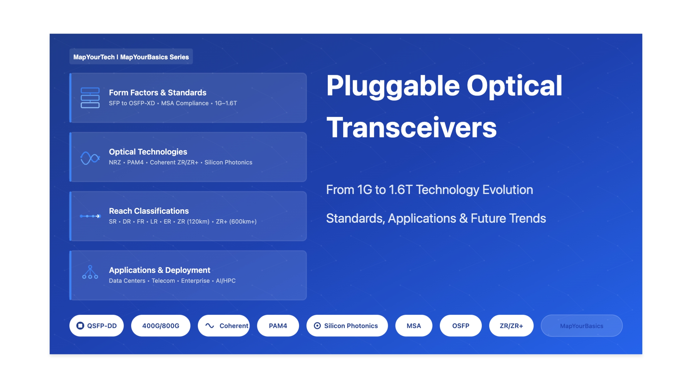
Complete Guide to Pluggable Optical Transceivers
Fundamentals & Core Concepts
What are Pluggable Optical Transceivers?
Pluggable optical transceivers are compact, hot-swappable network interface modules that serve as the critical bridge between electronic and optical domains in modern networks. These standardized devices convert electrical signals from network equipment (switches, routers, servers) into optical signals for transmission over fiber-optic cables, and vice versa.
Core Definition: An optical transceiver is a ubiquitous and essential component within modern packet networks, defined as a compact, hot-pluggable module whose core function is the efficient bidirectional conversion between electrical signals (used by the host ASIC or processor) and optical signals (transmitted over fiber optic cable).
The architecture of a pluggable transceiver comprises three main functional areas:
- Optoelectronic Devices: Laser transmitters (VCSELs, DFB lasers) and photodetectors for light generation and reception
- Functional Circuits: Digital Signal Processors (DSPs), laser drivers, clock-data recovery circuits, and signal conditioning electronics
- Optical Interface: Physical connectors (LC, MPO, CS) where fiber cables attach
Why Do They Exist?
Pluggable transceivers emerged from several critical industry needs:
1. Flexibility and Modularity
Unlike fixed optics integrated into equipment, pluggable modules allow network operators to:
- Choose the right transceiver for each link's specific needs (distance, speed, fiber type)
- Upgrade network capacity by simply swapping modules rather than replacing entire switches
- Maintain spare inventory that works across multiple equipment types
- Hot-swap modules without taking down the entire system
2. Standardization and Interoperability
Multi-Source Agreements (MSAs) ensure that transceivers from different manufacturers work seamlessly in any compliant host equipment. This prevents vendor lock-in and fosters competitive pricing.
3. Cost Optimization
The pay-as-you-grow model allows organizations to populate ports only as needed, avoiding upfront capital expenditure on unused capacity. The competitive multi-vendor ecosystem drives down prices through economies of scale.
When Does It Matter?
Pluggable transceivers are critical in scenarios requiring:
- High-density connectivity: Data centers with thousands of server connections
- Distance flexibility: From 2-meter copper DAC cables to 3,000+ km coherent optical links
- Rapid deployment: Cloud infrastructure scaling and network expansions
- Future-proofing: Equipment that needs to support multiple generations of technology
- Multi-vendor environments: Networks using equipment from various manufacturers
Why Is It Important?
Market Significance: The global optical transceiver market is projected to reach $36.73 billion by 2031, growing at a CAGR of 14.2%. This growth is driven by exponential data traffic increases, AI/ML workload demands, 5G infrastructure deployment, and the transition to 400G/800G networks.
Key importance factors:
- Enabling Cloud Computing: Every byte of data moving through cloud infrastructure passes through pluggable transceivers
- AI Infrastructure: Training large language models requires massive interconnect bandwidth, with 800G transceivers becoming standard
- 5G Networks: Mobile infrastructure relies on high-speed transceivers for fronthaul and backhaul connections
- Energy Efficiency: Modern transceivers optimize power per bit, reducing operational costs in large deployments
- Investment Protection: Standardized interfaces ensure that infrastructure investments remain relevant across technology generations
Mathematical Framework & Performance Calculations
Core Performance Formulas
Formula: Data Rate = Number of Lanes × Lane Speed
Example: QSFP-DD 400G module:
Data Rate = 8 lanes × 50 Gbps (PAM4) = 400 Gbps
Variables:
- Number of Lanes: Electrical channels (1, 4, 8, or 16)
- Lane Speed: Per-channel data rate (10, 25, 50, 100, 112 Gbps)
Formula: Link Budget (dB) = Tx Power (dBm) - Rx Sensitivity (dBm) - System Margin (dB)
Example: 100GBASE-LR4 link:
- Tx Power: -4.3 dBm (minimum)
- Rx Sensitivity: -10.6 dBm (maximum)
- Required System Margin: 2 dB
- Available Loss Budget: -4.3 - (-10.6) - 2 = 4.3 dB
Maximum Distance: Determined by fiber attenuation
Distance = Link Budget / Fiber Attenuation
For SMF @ 1310nm (0.4 dB/km): 4.3 dB / 0.4 dB/km ≈ 10.75 km
Formula: Power per Bit = Module Power (W) / Data Rate (Gbps)
Example Comparison:
| Module Type | Power | Data Rate | Power per Bit |
|---|---|---|---|
| 100G QSFP28 SR4 | 3.5 W | 100 Gbps | 35 mW/Gbps |
| 400G QSFP-DD DR4 | 12 W | 400 Gbps | 30 mW/Gbps |
| 800G OSFP DR8 | 14 W | 800 Gbps | 17.5 mW/Gbps |
Observation: Higher-speed modules generally achieve better power efficiency (lower mW/Gbps)
Formula: Maximum Ports = Available Faceplate Width / Module Width
Example: 1U (1.75") switch faceplate ≈ 17" usable width:
- SFP/SFP+: 17" / 0.54" ≈ 31 ports × 10G = 310 Gbps aggregate
- QSFP28: 17" / 0.68" ≈ 25 ports × 100G = 2.5 Tbps aggregate
- QSFP-DD: 17" / 0.71" ≈ 24 ports × 400G = 9.6 Tbps aggregate
- QSFP-DD800: 24 ports × 800G = 19.2 Tbps aggregate
Formula: Dispersion (ps/nm) = Dispersion Coefficient (ps/nm·km) × Distance (km)
Example: 100G transmission over 10 km of SMF:
- Standard SMF @ 1310nm: D = 0 ps/nm·km (zero-dispersion wavelength)
- Standard SMF @ 1550nm: D = 17 ps/nm·km
- Dispersion over 10 km @ 1550nm = 17 × 10 = 170 ps/nm
Mitigation: PAM4 and coherent modulation with DSP-based equalization can compensate for chromatic dispersion, enabling longer reach without dispersion compensation modules.
Practical Calculation Example: Link Design
Scenario: Design a 400G link between two data center buildings 2 km apart
Requirements:
- Distance: 2 km
- Data Rate: 400 Gbps
- Fiber: Single-mode OS2
- Budget: Cost-effective solution
Solution: 400GBASE-FR4
Calculations:
- Reach Capability: FR4 supports up to 2 km ✓
- Link Budget:
- Fiber loss: 2 km × 0.4 dB/km = 0.8 dB
- Connector loss: 2 connections × 0.5 dB = 1.0 dB
- Total loss: 1.8 dB
- FR4 loss budget: ~4.5 dB ✓
- Margin: 4.5 - 1.8 = 2.7 dB ✓
- Power Consumption: ~12W per module
- Cost Analysis: FR4 < LR4 (no CWDM required)
Result: 400GBASE-FR4 QSFP-DD modules with duplex LC connectors provide optimal cost-performance for this application.
Types, Form Factors & Component Breakdown
Evolution of Form Factors
Optical transceiver form factors have evolved continuously from the 1990s to support increasing data rates while maintaining or reducing physical size. Each form factor is standardized through Multi-Source Agreements (MSAs) that define mechanical, electrical, and thermal specifications.
1. SFP Family (Small Form-Factor Pluggable)
SFP (1G): Introduced in early 2000s, 1 Gbps, single lane, ~13.4mm × 8.5mm × 56.5mm
- Applications: Gigabit Ethernet, 1G/2G Fibre Channel
- Power: 0.5-1W
- Connectors: LC duplex (fiber), RJ45 (copper)
- Wavelengths: 850nm (MMF), 1310nm/1550nm (SMF)
SFP+ (10G): Same physical size as SFP, 10 Gbps, NRZ modulation
- Applications: 10 Gigabit Ethernet, 8G/16G Fibre Channel
- Power: 1-1.5W
- Reach: SR (100m MMF), LR (10km SMF), ER (40km SMF), ZR (80km SMF)
SFP28 (25G): Backward compatible form factor, 25 Gbps per lane
- Applications: 25 Gigabit Ethernet, 32G Fibre Channel
- Power: 1-2W
- Key Feature: Building block for 100G (4×25G) and server connectivity
SFP56 (50G): 50 Gbps PAM4 in SFP form factor
- Applications: 50 Gigabit Ethernet, 64G Fibre Channel
- Power: 2-3W
SFP-DD (100-200G): Double-density SFP with dual-row connector
- Configuration: 2 lanes × 50G PAM4 = 100G, or 2 × 100G PAM4 = 200G
- Power: 2.5-4W
- Status: Emerging for high-density 100G applications
2. QSFP Family (Quad Small Form-Factor Pluggable)
QSFP+ (40G): Four lanes at 10 Gbps each, ~18mm × 72mm × 8.5mm
- Applications: 40 Gigabit Ethernet, 4×10G breakout
- Power: 3.5W
- Connectors: MPO-12 (parallel fiber), LC duplex (CWDM4)
QSFP28 (100G): Four lanes at 25 Gbps each (NRZ)
- Applications: 100 Gigabit Ethernet, 100G InfiniBand EDR
- Power: 3.5-5W
- Variants: SR4 (MMF 100m), PSM4 (SMF 500m), LR4 (SMF 10km), ER4 (SMF 40km)
- Market Dominance: Most widely deployed 100G form factor
QSFP56 (200G): Four lanes at 50 Gbps each (PAM4)
- Applications: 200 Gigabit Ethernet, 200G InfiniBand HDR
- Power: 6-12W
- Usage: Intermediate step, some adoption in 2×100G breakout scenarios
QSFP-DD (400-800G): Double-density with 8 lanes, backward compatible
- Configuration 1: 8 lanes × 50G PAM4 = 400G
- Configuration 2: 8 lanes × 100G PAM4 = 800G
- Power: 12W (400G), 14W (800G)
- Key Advantage: Fits in similar footprint to QSFP28, allowing high port density (36×400G in 1U)
- Connectors: MPO-12/16, dual LC, dual CS
- Status: Dominant 400G form factor, rapidly scaling to 800G
QSFP112 (400G): Four lanes at 112 Gbps each
- Configuration: 4 × ~112G PAM4 = 400G
- Status: Limited adoption, primarily discussed for InfiniBand NDR
- Challenge: Signal integrity at 112G over QSFP connector
3. OSFP Family (Octal Small Form-Factor Pluggable)
OSFP (400-800G): Eight lanes, designed for high thermal performance
- Dimensions: ~22.6mm × 107.2mm × 13mm (larger than QSFP-DD)
- Configuration 1: 8 × 50G PAM4 = 400G
- Configuration 2: 8 × 100G PAM4 = 800G
- Power: 15-20W (integrated heatsink provides superior thermal management)
- Key Advantage: Better cooling for high-power coherent and 800G modules
- Compatibility: Not backward compatible with QSFP (requires adapter)
- Adoption: Favored by hyperscalers (Meta/Facebook) and for future 1.6T
OSFP-XD (1.6T): Extended Depth variant for next-generation speeds
- Configuration: 16 lanes × 100G or 8 lanes × 200G = 1.6 Tbps
- Power: 25-30W
- Status: Development stage, expected commercial availability 2025-2026
4. Legacy and Specialized Form Factors
GBIC (Gigabit Interface Converter): First hot-pluggable standard, 1 Gbps
- Era: Late 1990s - early 2000s
- Status: Obsolete, replaced by smaller SFP
XENPAK, X2, XPAK (10G): Early 10G modules
- Characteristics: Large size (SC or MPO connectors)
- Status: Obsolete, replaced by XFP and SFP+
XFP (10G): 10 Gigabit small form factor
- Features: LC duplex, protocol-independent
- Status: Largely replaced by SFP+ (smaller, lower power)
CFP Family (100-400G): C Form-Factor Pluggable (C=100 in Roman numerals)
- CFP: Large module for 100G, primarily coherent
- CFP2: Half the size of CFP, widely used for 100G/200G coherent (CFP2-DCO)
- CFP4: Quarter size of CFP, 100G
- CFP8: 400G variant
- Power: 20-32W (allows high-power coherent DSPs)
- Status: Declining, replaced by QSFP-DD/OSFP for most applications
- Remaining Use: Long-haul optical transport networks
Form Factor Comparison Table
| Form Factor | Lanes | Max Speed | Power | Size (W×L) | Status |
|---|---|---|---|---|---|
| SFP | 1 | 1G | 1W | 13.4×56.5mm | Legacy |
| SFP+ | 1 | 10G | 1.5W | 13.4×56.5mm | Mature |
| SFP28 | 1 | 25G | 2W | 13.4×56.5mm | Current |
| SFP56 | 1 | 50G | 3W | 13.4×56.5mm | Current |
| SFP-DD | 2 | 200G | 4W | 13.4×56.5mm | Emerging |
| QSFP+ | 4 | 40G | 3.5W | 18×72mm | Mature |
| QSFP28 | 4 | 100G | 5W | 18×72mm | Current |
| QSFP56 | 4 | 200G | 12W | 18×72mm | Current |
| QSFP-DD | 8 | 800G | 14W | 18×72mm | Current/Growth |
| OSFP | 8 | 800G | 20W | 22.6×107mm | Current/Growth |
| OSFP-XD | 8-16 | 1.6T | 30W | 22.6×140mm | Development |
Reach Categories and Wavelengths
SR (Short Reach): Multimode fiber, 850nm VCSEL, 30-100m (OM3), 100-150m (OM4), ~150-400m (OM5)
Use Case: Intra-data center server-to-switch links, cost-effective for short distances
LR (Long Reach): Single-mode fiber, 1310nm DFB laser, typically 10 km
Use Case: Campus networks, inter-building data center links, metro access
ER (Extended Reach): Single-mode fiber, 1550nm laser, 30-40 km
Use Case: Metro networks, regional data center interconnects
ZR/ZR+ (Zero-Dispersion/Extended): Single-mode fiber, coherent technology, 80-120 km (ZR), 600+ km (ZR+)
Use Case: Data center interconnect, metro/regional networks, long-haul transport
DR (Data Center Short Reach): Single-mode fiber, 1310nm, 500m
Use Case: Optimized for data center row-to-row and building-to-building connections
FR (Fiber Reach): Single-mode fiber, CWDM/LAN-WDM, 2 km
Use Case: Data center and campus networks, cost-effective alternative to LR4
Effects, Impacts & System Considerations
System-Level Performance Effects
1. Signal Integrity and Modulation Impact
NRZ (Non-Return-to-Zero) Modulation:
- Characteristics: Two signal levels (0 and 1), simple implementation
- Speed Limits: Practical maximum ~28 Gbps per lane
- Power: Low consumption, minimal DSP required
- Applications: 10G, 25G, 40G, early 100G modules
- Limitation: Bandwidth requirements scale linearly with data rate
PAM4 (4-Level Pulse Amplitude Modulation):
- Characteristics: Four signal levels (00, 01, 10, 11), 2 bits per symbol
- Advantage: Doubles data rate without increasing bandwidth: 50 Gbps at 25 GBaud, 100 Gbps at 50 GBaud
- Trade-offs:
- Reduced SNR (closer signal levels increase noise susceptibility)
- Higher BER without FEC
- Requires sophisticated DSP and equalization
- Increased power consumption (12-15W for 800G modules)
- Applications: 200G, 400G, 800G modules standard
Coherent Modulation (QPSK, QAM):
- Characteristics: Encodes data in amplitude, phase, and dual polarization
- Performance: Enables 400G-800G over 120+ km without amplification
- Trade-offs:
- Very high power (15-25W per module)
- Complex DSP required
- Higher cost
- Applications: Data center interconnect, metro/long-haul networks, 400ZR/ZR+ standard
2. Power and Thermal Management Impact
Critical Challenge: At 800G speeds with PAM4 modulation, each module can consume 14-20W. A fully loaded 36-port QSFP-DD switch can draw 504-720W just from transceivers, creating significant thermal challenges.
Thermal Management Strategies:
- QSFP-DD Approach: Riding heatsink on host switch, relies on high airflow (requires powerful cooling fans)
- OSFP Approach: Integrated heatsink within module, better heat spreading, allows higher power modules
- LPO (Linear Pluggable Optics): Removes DSP from module, reduces power by 30-40%, but requires high-quality electrical traces on host
Power Efficiency Trends:
| Generation | Module Example | Power per Gbps | Trend |
|---|---|---|---|
| 10G | SFP+ SR | 150 mW/Gbps | Baseline |
| 100G | QSFP28 SR4 | 35 mW/Gbps | 77% improvement |
| 400G | QSFP-DD DR4 | 30 mW/Gbps | 14% improvement |
| 800G | OSFP DR8 | 17.5 mW/Gbps | 42% improvement |
3. Density and Port Count Impact
Economic Impact of Port Density:
- Capital Efficiency: QSFP-DD enables 36×400G = 14.4 Tbps in 1U, reducing datacenter space requirements
- Cable Management: Higher port count increases complexity of fiber management
- Breakout Flexibility: One 400G port can breakout to 4×100G, providing deployment flexibility
4. Latency Considerations
DSP-Induced Latency:
- PAM4 with DSP: Adds 200-500ns per hop (FEC encoding/decoding, equalization)
- Coherent Modules: Can add 1-2 microseconds due to complex DSP processing
- LPO Modules: Minimal latency (<50ns), critical for high-frequency trading and low-latency applications
- Impact: In a 5-hop network, DSP latency can accumulate to 1-2.5 microseconds
5. Fiber Infrastructure Impact
| Impact Area | MMF (Multimode) | SMF (Single-Mode) |
|---|---|---|
| Cost | Lower (fiber + transceivers) | Higher initial, lower long-term |
| Distance | 30-400m depending on fiber grade | 2 km to 3,000+ km |
| Upgrade Path | Limited (OM3→OM4→OM5) | Excellent (supports multiple generations) |
| Modal Dispersion | Significant (limits bandwidth×distance) | Minimal (chromatic only) |
| Best Use | Intra-building data centers | Campus, metro, long-haul |
Operational Impact Analysis
6. Total Cost of Ownership (TCO) Impact
5-Year TCO Breakdown for 1000-Port Data Center:
- Capital Expenditure:
- Transceivers: $500-$2,000 per port depending on speed/reach
- Switch equipment: Amortized over transceiver lifetime
- Cabling infrastructure: $50-$200 per link
- Operational Expenditure:
- Power consumption: $100-$300 per port annually (at $0.10/kWh)
- Cooling costs: 0.5-1× power consumption cost
- Maintenance: 5-10% of CapEx annually
- Failure replacement: 1-2% annual failure rate
7. Supply Chain and Availability Impact
Market Dynamics:
- Lead Times: Standard modules (2-4 weeks), coherent/specialized (8-12 weeks), custom variants (16+ weeks)
- Price Volatility: 10-30% variation based on demand spikes and component shortages
- Multi-Sourcing: MSA standardization enables multiple suppliers, reducing risk
- Geopolitical Risk: 80%+ manufacturing in Asia (China, Taiwan, Malaysia), diversification ongoing
8. Interoperability and Standards Compliance
Positive Impacts:
- MSA compliance ensures multi-vendor compatibility
- Reduces vendor lock-in and procurement costs
- Simplifies spare parts inventory management
- Enables competitive bidding processes
Challenges:
- Some vendors use proprietary encoding in EEPROM for "genuine" detection
- Warranty concerns with third-party transceivers
- Feature compatibility (DDM, temperature ranges) may vary
Implementation Techniques & Technology Solutions
1. Silicon Photonics Technology
What It Is: Integration of optical components (waveguides, modulators, detectors) on silicon substrates using CMOS-compatible processes
Key Advantages:
- Cost Reduction: Leverages existing semiconductor manufacturing infrastructure, enabling mass production
- Size Miniaturization: Integrates multiple optical functions on single chip
- Performance: Enables high-speed modulation and low-loss waveguides
- Scalability: Moore's Law benefits apply to photonic integration
Applications:
- 400G/800G transceiver optical engines
- Coherent DSP-integrated photonic circuits
- WDM multiplexers/demultiplexers on chip
Market Impact: Silicon photonics market growing at 25%+ CAGR, driving down costs of high-speed transceivers by 20-30% per generation
2. DSP-Based Signal Processing Techniques
Equalization and Pre-Compensation:
- Feed-Forward Equalization (FFE): Compensates for channel loss and ISI
- Decision Feedback Equalization (DFE): Reduces post-cursor interference
- Pre-Emphasis: Boosts high-frequency components at transmitter
- Effect: Enables reliable transmission over longer copper traces and lower-quality fiber
Forward Error Correction (FEC):
- RS-FEC (Reed-Solomon): IEEE 802.3 standard for 100G/400G
- KP4-FEC: Higher overhead (20-25%), better correction for coherent links
- o-FEC (OpenFEC): Optimized for 400ZR applications
- Benefit: Allows operation at higher BER, extending reach and relaxing component requirements
- Trade-off: Adds latency (200-500ns) and increases data overhead
3. Advanced Connector Technologies
| Connector | Type | Fibers | Applications | Advantages |
|---|---|---|---|---|
| LC Duplex | Single-mode | 2 | 10G-400G LR/ER optics | Standard, reliable, small footprint |
| MPO-12 | Multi-fiber | 12 | 40G/100G SR4, breakouts | High density, parallel transmission |
| MPO-16 | Multi-fiber | 16 | 400G/800G SR8 | Supports 8-lane parallel optics |
| CS (Duplex) | Compact duplex | 2 | 200G/400G FR4 | Smaller than LC, enables breakouts |
| MDC (Multifiber) | Multi-fiber | 16-32 | 800G/1.6T future | Ultra-high density |
4. Power Optimization Techniques
LPO (Linear Pluggable Optics):
- Concept: Remove DSP from transceiver, perform equalization on host ASIC
- Power Savings: 30-40% reduction (800G LPO: ~9W vs. standard 14W)
- Requirements: High-quality PCB traces, advanced host-side SerDes
- Trade-offs: Shorter reach capability, less link flexibility
- Best For: Short-reach data center applications with controlled environments
Dynamic Power Management:
- Automatic power-down of unused lanes in breakout scenarios
- Adaptive transmit power based on link budget requirements
- Sleep modes for idle periods (energy-efficient ethernet)
- Thermal-based throttling to prevent overheating
5. Co-Packaged Optics (CPO) - Emerging Solution
Concept: Integrate optical transceivers directly onto the same package as the switch ASIC, eliminating long electrical traces and front-panel constraints
Advantages:
- Power Efficiency: 30% reduction by eliminating retimers and long SerDes lanes
- Density: Enables switch ASICs with 100+ terabits aggregate capacity
- Signal Integrity: Shorter electrical paths reduce loss and EMI
- Latency: 10-20% reduction vs. pluggable modules
Challenges:
- Serviceability: Cannot hot-swap individual optics, entire package replacement required
- Standardization: Lack of MSA-level standards (OIF working on specifications)
- Vendor Lock-in: Proprietary interfaces between ASIC and optical engine
- Manufacturing Complexity: Requires co-design of silicon and photonics
- Thermal Management: Heat from ASIC affects optical components
Status: Early adoption in hyperscale AI clusters (NVIDIA, Broadcom demos), mainstream deployment expected 2027-2030
6. Coherent Technology Solutions
DCO (Digital Coherent Optics) Architecture:
- Integration: Full DSP integrated in transceiver module
- Interface: Digital communication with host (Ethernet frames)
- Advantages: Plug-and-play simplicity, dynamic reconfiguration
- Applications: 400ZR, 400ZR+, 800ZR standards
ACO (Analog Coherent Optics) Architecture:
- Integration: DSP on host line card, optical analog interface
- Interface: Analog I/Q signals
- Advantages: Higher performance ceiling for specialized applications
- Applications: Long-haul optical transport (legacy)
- Status: Being phased out in favor of DCO
7. Wavelength Division Multiplexing (WDM) Techniques
CWDM (Coarse WDM):
- Channel Spacing: 20nm (ITU-T G.694.2)
- Typical Wavelengths: 1271nm, 1291nm, 1311nm, 1331nm for CWDM4
- Cost: Lower (uncooled lasers acceptable)
- Applications: 100G-LR4, 400G-FR4 short-medium reach
LAN-WDM:
- Channel Spacing: ~800 GHz (~6.5nm)
- Advantage: Denser than CWDM, more channels on single fiber
- Applications: 400G-FR8, data center optimized
DWDM (Dense WDM):
- Channel Spacing: 50-100 GHz (ITU-T G.694.1)
- Typical Grid: 96 channels in C-band (1530-1565nm)
- Requirements: Cooled, tunable lasers with tight wavelength control
- Applications: Coherent 400ZR/ZR+, long-haul transport, metro networks
Implementation Best Practices
| Practice | Description | Benefit |
|---|---|---|
| Fiber Grade Selection | Use OM4/OM5 for MMF, OS2 for SMF new installations | Future-proofs infrastructure for speed upgrades |
| Structured Cabling | Implement MTP/MPO trunk cables with LC breakout cassettes | Simplifies moves/adds/changes, reduces labor |
| Thermal Monitoring | Use DDM/DOM features to track module temperature | Prevents thermal throttling, predicts failures |
| Power Budgeting | Calculate total transceiver power before deployment | Ensures adequate PSU and cooling capacity |
| Multi-Vendor Testing | Validate third-party transceivers in lab before production | Reduces risk, ensures compatibility |
| Spare Strategy | Stock 5-10% spares of each critical transceiver type | Minimizes downtime during failures |
| Cleaning Protocol | Clean all fiber connectors before mating | Prevents contamination-related failures |
| Documentation | Maintain database of module serial numbers, locations | Enables failure analysis, warranty tracking |
Design Guidelines & Selection Methodology
Step-by-Step Transceiver Selection Process
Step 1: Define Requirements
Key Questions to Answer:
- Required Data Rate: What speed per port? (1G, 10G, 25G, 100G, 400G, 800G)
- Link Distance: Maximum cable length required?
- Fiber Type Available: Multimode (OM3/OM4/OM5) or Single-mode (OS2)?
- Port Density Needs: How many ports per switch/rack unit?
- Budget Constraints: What is cost per port target?
- Power Limitations: Available power and cooling capacity?
- Environmental Factors: Temperature range, humidity, vibration?
- Protocol Support: Ethernet, Fibre Channel, InfiniBand, OTN?
- Latency Requirements: Ultra-low latency critical? (trading, HPC)
- Future Scalability: Upgrade path considerations?
Step 2: Select Form Factor
If Data Rate ≤ 25G: → SFP/SFP+/SFP28 family
If Data Rate = 40-50G: → QSFP+/QSFP28/SFP56
If Data Rate = 100G: → QSFP28 (most common) or SFP-DD (high density)
If Data Rate = 200G: → QSFP56 or SFP-DD
If Data Rate = 400G: → QSFP-DD (backward compatible) or OSFP (thermal headroom)
If Data Rate = 800G: → QSFP-DD or OSFP (OSFP preferred for coherent)
If Data Rate ≥ 1.6T: → OSFP-XD (future)
Additional Considerations:
- Existing Infrastructure: If QSFP ports exist, QSFP-DD provides backward compatibility
- Power Budget: If power is constrained, favor QSFP-DD over OSFP
- Future 800G+ Plans: If planning 800G+ migration, OSFP offers better thermal headroom
Step 3: Determine Reach Classification
| Distance Requirement | Fiber Type | Reach Classification | Typical Wavelength |
|---|---|---|---|
| 0-100m (intra-rack, row-to-row) | Multimode OM3/OM4 | SR (Short Reach) | 850nm VCSEL |
| 100-300m (building) | Multimode OM4/OM5 or SMF | SR (OM5) or PSM4/DR | 850nm or 1310nm |
| 300-500m (campus) | Single-mode | DR4 (500m optimized) | 1310nm |
| 500m-2km (campus, multi-building) | Single-mode | FR4/FR8 | CWDM4 or LAN-WDM |
| 2-10km (metro access) | Single-mode | LR4/LR8 | CWDM4 or DWDM |
| 10-40km (metro) | Single-mode | ER4 | 1550nm |
| 40-120km (metro/regional DCI) | Single-mode | ZR (coherent) | Tunable C-band DWDM |
| >120km (long-haul) | Single-mode | ZR+/ULH (coherent) | Tunable C-band DWDM |
Step 4: Calculate Link Budget
Given Parameters:
- Tx Min Power: __________ dBm (from transceiver datasheet)
- Rx Sensitivity: __________ dBm (from transceiver datasheet)
- Link Distance: __________ km
- Fiber Attenuation: __________ dB/km (0.35 @ 1310nm, 0.25 @ 1550nm typical)
- Number of Connectors: __________ (2 typical for point-to-point)
- Connector Loss: 0.5 dB each (typical)
- Number of Splices: __________ (if applicable)
- Splice Loss: 0.1 dB each (typical)
Calculation:
- Available Power Budget = Tx Min Power - Rx Sensitivity = __________ dB
- Fiber Loss = Distance × Attenuation = __________ dB
- Connector Loss = Number of Connectors × 0.5 dB = __________ dB
- Splice Loss = Number of Splices × 0.1 dB = __________ dB
- Total Path Loss = Fiber + Connector + Splice = __________ dB
- System Margin = Available Budget - Total Path Loss = __________ dB
Evaluation:
- Margin > 3 dB: Excellent
- Margin 2-3 dB: Good
- Margin 1-2 dB: Marginal
- Margin < 1 dB: Insufficient
Step 5: Evaluate Cost-Performance Trade-offs
Example Scenario: 100 Gbps link, 5 km distance
| Option | Transceiver Cost | Fiber Req. | Power | Total 5-Year TCO |
|---|---|---|---|---|
| 100G-SR4 + Fiber conversion | $300 × 2 = $600 | MMF→SMF converters | 7W | $1,800 |
| 100G-LR4 | $1,200 × 2 = $2,400 | OS2 SMF (existing) | 5W | $2,900 |
| 100G-PSM4 | $600 × 2 = $1,200 | OS2 SMF (4 fibers) | 4.5W | $1,900 |
Winner: 100G-PSM4 - Best TCO balance for this scenario
Step 6: Consider Environmental Factors
Operating Temperature Ranges:
- Commercial (0°C to 70°C): Standard data center transceivers
- Industrial (-40°C to 85°C): Outdoor deployments, 5G fronthaul, harsh environments
- Extended (0°C to 85°C): Intermediate option for telecom
Additional Environmental Considerations:
- Humidity: Most transceivers rated 5-85% RH non-condensing
- Altitude: Standard rating up to 3,000m; derating may be required for higher elevations
- EMI/EMC: FCC Class A/B compliance for different environments
- Vibration/Shock: Telecom-grade specifications for mobile applications
Common Design Pitfalls to Avoid
| Pitfall | Impact | Prevention |
|---|---|---|
| Under-budgeting power | Thermal throttling, system instability | Calculate worst-case power (all ports populated, full load) |
| Mixing multimode grades | Reduced performance on lowest-grade fiber | Document and maintain consistent fiber infrastructure |
| Ignoring connector quality | High insertion loss, reliability issues | Use quality connectors, implement cleaning protocols |
| Not testing third-party modules | Compatibility issues, warranty concerns | Lab test before production deployment |
| Insufficient cooling airflow | Module overheating, early failures | Follow vendor airflow specifications, monitor temperatures |
| Over-specifying reach | Unnecessary cost | Use link budget calculations to select appropriate reach |
| No upgrade path planning | Costly infrastructure replacement | Install OS2 SMF for future-proofing, even if using MMF initially |
Design Decision Matrix
Use this matrix to guide transceiver selection:
| Priority | Optimization Strategy | Recommended Approach |
|---|---|---|
| Lowest CapEx | Minimize upfront cost | Third-party modules, MMF where possible, SR optics |
| Lowest TCO | Optimize 5-year total cost | Balance CapEx with power efficiency, plan for growth |
| Maximum Density | Most ports per RU | SFP28 (single-width) or QSFP-DD (high aggregate) |
| Best Performance | Lowest latency, highest reliability | OEM modules, LPO for latency, quality fiber infrastructure |
| Future-Proofing | Long-term flexibility | OS2 fiber, QSFP-DD form factor, plan for 2× speed growth |
| Simplicity | Easy deployment & support | Single vendor, common modules, extensive documentation |
Interactive Simulators & Calculators
Understanding Reach Classifications
Before using the simulators, it's important to understand the reach type designations:
- SR (Short Reach): Optimized for multimode fiber, typically 30-150m using 850nm VCSELs
- DR (Data Center Reach): Designed for 500m over single-mode fiber at 1310nm, perfect for intra-campus
- FR (Fiber Reach): 2km capability using CWDM/LAN-WDM wavelengths on single-mode fiber
- LR (Long Reach): Standard 10km solution for metro access and campus networks
- ER (Extended Reach): 40km capability for metro and regional networks
- ZR (Zero-dispersion Reach): 80-120km coherent technology optimized for the zero-dispersion region, enabling long-haul data center interconnect without amplification
- ZR+ (Extended Zero-dispersion Reach): Enhanced coherent solution reaching 600+ km with amplification, for ultra-long-haul applications
Note on ZR Technology: The "ZR" designation refers to operation in the zero-dispersion region of optical fiber (around 1310nm for standard SMF, or C-band with dispersion compensation). Coherent ZR/ZR+ transceivers use advanced modulation (DP-QPSK, DP-16QAM) and integrated DSPs to achieve remarkable distances while maintaining the pluggable form factor. This technology has revolutionized data center interconnect by eliminating the need for separate transponder equipment.
📍 Recommended Transceiver:
Alternative Options:
Reach Classification Guide:
Practical Applications & Real-World Case Studies
Primary Application Segments
1. Data Center Interconnects (DCI)
Intra-Data Center Applications:
- Server-to-ToR (Top of Rack): 25G/50G/100G SFP28/QSFP28 SR modules, typically 10-30m links using OM4 MMF or copper DAC
- ToR-to-Spine: 100G/400G QSFP28/QSFP-DD, 50-100m using OM4/OM5 MMF or OS2 SMF
- Spine-to-Spine: 400G/800G QSFP-DD/OSFP for leaf-spine fabrics in mega data centers
- AI/ML Clusters: 400G/800G with ultra-low latency for GPU-to-GPU communication
Inter-Data Center (Campus/Metro DCI):
- Building-to-Building: 100G/400G LR4/FR4 for 2-10km using OS2 SMF
- Metro DCI: 400G ZR/ZR+ coherent pluggables for 10-120km between facilities
- Regional DCI: 400G ZR+ supporting 600+ km with amplification
Market Impact: Data center applications represent the largest segment of transceiver demand, driven by cloud computing growth and AI infrastructure buildout.
2. Enterprise Networking
Campus Networks:
- Distribution/Access: 1G/10G SFP/SFP+ for connecting buildings across campus, typically 100m-2km
- Core Switches: 40G/100G QSFP+/QSFP28 for aggregating traffic
- Storage Networks (SAN): 8G/16G/32G Fibre Channel SFP+/SFP28 connecting to storage arrays
Deployment Characteristics:
- Typically one generation behind hyperscalers (10G/25G/100G most common)
- Emphasis on reliability and vendor support over cutting-edge performance
- Mix of MMF (existing infrastructure) and SMF (new deployments)
- Cost-sensitive, often use third-party transceivers for savings
3. Telecommunications & Service Provider Networks
5G Infrastructure:
- Fronthaul: 25G SFP28 connecting RRUs (Remote Radio Units) to baseband, industrial temp rating (-40°C to 85°C)
- Midhaul/Backhaul: 100G QSFP28 aggregating 5G traffic back to core
- Mobile Edge Computing: 100G/400G for low-latency connections to edge data centers
Metro/Core Networks:
- IP/MPLS Routers: 100G/400G coherent pluggables (CFP2-DCO, QSFP-DD ZR) enabling IP over DWDM
- Optical Transport (OTN): Legacy CFP/CFP2 for long-haul, transitioning to pluggable coherent
- Access Networks: 1G/10G SFP+ for GPON, XGS-PON OLT (Optical Line Terminals)
Trend: Telecom shifting from dedicated transponders to router-integrated coherent pluggables, reducing power and space while improving agility.
4. High-Performance Computing (HPC) & AI
Requirements:
- Ultra-High Bandwidth: 400G/800G standard, 1.6T emerging for GPU interconnects
- Ultra-Low Latency: LPO modules preferred to minimize DSP-induced latency
- Massive Scale: Thousands of transceivers in single cluster (e.g., 10,000-node AI training cluster = 40,000+ optical links)
- Reliability: Mission-critical, any failure impacts expensive compute time
Applications:
- GPU-to-GPU: Direct optical connections for distributed training workloads
- Storage Interconnect: High-speed access to distributed file systems
- Cluster Networking: Multi-tier Clos or dragonfly topologies
Case Study 1: Hyperscale Cloud Provider - 400G Data Center Upgrade
Challenge:
A major cloud provider needed to upgrade their data center network from 100G to 400G to support growing AI workloads. The existing infrastructure had QSFP28 ports and OS2 single-mode fiber plant with 80-300m link distances.
Requirements:
- Upgrade to 400G without replacing switches
- Minimize power consumption (cooling costs significant)
- Maintain backward compatibility during migration
- Cost target: <$1,000 per 400G transceiver
Solution Approach:
- Form Factor Selection: QSFP-DD chosen for backward compatibility with existing QSFP28 ports
- Reach Analysis:
- 80% of links <100m → considered SR8 on MMF but existing fiber is SMF
- Selected 400G-DR4 (500m capability using 4×100G PAM4 on parallel SMF)
- Power Optimization: Specified LPO DR4 modules where possible (9W vs. 12W standard)
- Phased Migration:
- Phase 1: Upgrade spine-to-spine links to 400G
- Phase 2: Upgrade leaf-to-spine
- Phase 3: Maintain 100G at leaf-to-server during servers' refresh cycle
- Vendor Strategy: Dual-sourced from qualified third-party suppliers achieving $750/module pricing
Results:
- Performance: 4× capacity increase, supporting 3× growth in AI training workloads
- Cost: $35M transceiver spend for 10,000-port deployment, 25% below OEM pricing
- Power: LPO modules saved 30W per link × 5,000 links = 150kW total, $131k annual savings
- Timeline: 18-month migration completed without network downtime
- Lessons: Existing fiber infrastructure critical - OS2 plant enabled smooth upgrade path
Case Study 2: Financial Services - Low-Latency Trading Network
Challenge:
A high-frequency trading firm needed to connect their trading servers to exchange co-location facilities with absolute minimum latency. Every microsecond of latency impacts trading profitability.
Requirements:
- Distance: 0.5 - 15 km (within metro area)
- Data Rate: 100G per trading server
- Latency: Absolute minimum (target <2μs end-to-end)
- Reliability: 99.999% uptime requirement
Solution Approach:
- Transceiver Selection:
- Rejected standard 100G QSFP28 LR4 (DSP adds 300-500ns latency per hop)
- Selected specialized low-latency 100G BiDi (bidirectional on single fiber)
- Total transceiver latency: <50ns vs. 400ns for standard module
- Fiber Infrastructure:
- Dedicated dark fiber leased for each route
- Multiple diverse paths for redundancy
- Ultra-low latency cables (reduced refractive index)
- Network Design:
- Direct server-to-exchange connections (no intermediate switches where possible)
- Where switches required, cut-through forwarding mode
- Precision time protocol (PTP) synchronization
Results:
- Latency: Achieved 1.8μs average end-to-end (fiber + transceiver + switch)
- Performance: 350ns improvement vs. standard transceiver solution
- Cost: $3,500 per specialized transceiver (3.5× standard LR4), justified by trading advantage
- Reliability: Zero fiber cuts in 2 years, hot-spare transceivers on-site for rapid swap
- ROI: Latency improvement enabled additional $12M annual trading profit
Case Study 3: Telecom Operator - 5G Fronthaul Deployment
Challenge:
A national telecom operator deploying 5G infrastructure needed transceivers for fronthaul connections between centralized baseband units (BBU) and remote radio units (RRU) on cell towers. Harsh outdoor environment and cost constraints were primary concerns.
Requirements:
- Data Rate: 25G per RRU (eCPRI/RoE protocol)
- Distance: 1-20 km (cell sites to central BBU pool)
- Environmental: Industrial temp -40°C to +85°C, outdoor-rated
- Volume: 50,000 cell sites over 3 years = 100,000+ transceivers
- Cost: Aggressive target due to massive volume
Solution Approach:
- Form Factor: 25G SFP28 (single-lane simplifies inventory, lower cost)
- Reach Selection:
- 10G BiDi for <10km (single fiber saves infrastructure cost)
- 25G LR for 10-20km where dual fiber available
- Industrial Hardening:
- Extended operating temperature SFP28 modules
- Conformal coating on PCBs for moisture resistance
- Enhanced ESD protection for outdoor deployment
- Procurement Strategy:
- Competitive bid among 5 qualified suppliers
- 3-year volume commitment for pricing leverage
- Achieved $150 per industrial-grade SFP28 (50% discount from initial quotes)
- Deployment Process:
- Pre-tested modules in controlled environment before field deployment
- Spares staged at regional distribution centers
- Remote diagnostics via DDM monitoring for proactive replacement
Results:
- Deployment: 85,000 modules deployed over 30 months
- Reliability: 0.8% annual failure rate (better than specified 1.5%)
- Cost: $12.75M total transceiver spend, 40% below budget
- Performance: <1ms latency supporting URLLC (Ultra-Reliable Low-Latency Communication)
- Operational Efficiency: DDM monitoring predicted 60% of failures before service impact
- Lessons: Volume commitment critical for pricing; field-testing essential for harsh environments
Troubleshooting Guide
| Symptom | Possible Causes | Diagnosis Steps | Solution |
|---|---|---|---|
| Link Down | Dirty connector, bad fiber, module failure, configuration mismatch | 1. Check LED status 2. Verify DDM values 3. Inspect connectors 4. Test with known-good module |
Clean connectors, replace fiber/module, verify speed/duplex settings |
| High Error Rate | Signal attenuation, dispersion, EMI, damaged fiber | 1. Check Rx power (should be within sensitivity range) 2. Verify FEC counters 3. Check for excessive link flaps |
Use shorter cable, add inline amplifier, check fiber bend radius, replace damaged fiber |
| Intermittent Failures | Thermal throttling, loose connector, marginal link budget | 1. Monitor module temperature 2. Check Rx power over time 3. Verify connector seating 4. Check for switch overheating |
Improve airflow, reseat connectors, use higher-power transceiver, add system margin |
| Module Not Recognized | Incompatible module, EEPROM issue, port failure | 1. Verify module compatibility list 2. Test in different port 3. Check for firmware updates |
Use compatible module, update switch firmware, RMA faulty port/module |
| Performance Degradation | Aging components, dirty optics, thermal drift | 1. Compare current vs. baseline DDM values 2. Check link utilization 3. Verify temperature trending |
Proactive module replacement, improve cooling, load balancing across links |
Quick Reference: Application Best Practices
Note: This guide is based on industry standards, best practices, and real-world implementation experiences. Specific implementations may vary based on equipment vendors, network topology, and regulatory requirements. Always consult with qualified network engineers and follow vendor documentation for actual deployments.
Unlock Premium Content
Join over 400K+ optical network professionals worldwide. Access premium courses, advanced engineering tools, and exclusive industry insights.
Already have an account? Log in here