Discover the best Q-factor improvement techniques for optical networks with this comprehensive guide. Learn how to optimize your network’s performance...
Q-factor Improvement Techniques for Optical Networks – Comprehensive Guide Q-factor Improvement Techniques for Optical Networks A Comprehensive Professional Guide to...
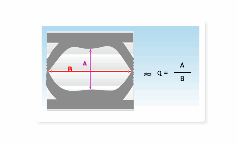
Understanding Q-Factor in Optical Communications Understanding Q-Factor in Optical Communications Comprehensive Signal Quality Metrics and Performance Analysis What is Q-Factor?...