Spectral Efficiency in Optical Networks

Admin November 4, 2025 No Comments Free Fundamentals Technical

6 min read

Spectral Efficiency Guide | MapYourTech

1. Fundamentals & Core Concepts

What is Spectral Efficiency?

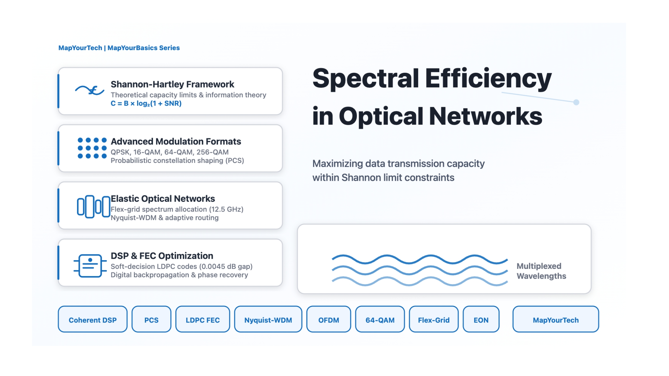
Spectral Efficiency (SE) is a fundamental performance metric in optical communications that quantifies how effectively the available optical spectrum is utilized to transmit information. It represents the information capacity transmitted per unit bandwidth, measured in bits per second per Hertz (bits/s/Hz).

SE = (R_s × log₂(M)) / (Δf × (1 + r))

Where: R_s = Symbol rate (baud), M = Constellation points, Δf = Channel spacing (Hz), r = FEC redundancy

Historical Evolution: The industry has progressed from ~0.4 bits/s/Hz (10G OOK, early 2000s) to 8-12 bits/s/Hz (800G-1.2T systems, 2025), but improvement rates are exponentially slowing as systems approach the Shannon limit.

Era	Data Rate	Modulation	SE	Key Technology
2010-2012	100 Gb/s	DP-QPSK	~2 bits/s/Hz	Coherent detection
2015-2018	200 Gb/s	DP-16QAM	~4 bits/s/Hz	Advanced DSP
2020-2022	400-600 Gb/s	DP-64QAM	~6-8 bits/s/Hz	PCS + SD-FEC
2023-2025	800G-1.2T	DP-64QAM/128QAM	~8-12 bits/s/Hz	5nm DSP, 120+ Gbaud

2. Mathematical Framework

Shannon-Hartley Theorem

The theoretical foundation for channel capacity derives from Claude Shannon's information theory, defining the maximum theoretical data rate for a bandwidth-limited channel with additive white Gaussian noise (AWGN).

C = B × log₂(1 + SNR)

Where: C = Channel capacity (bits/s), B = Bandwidth (Hz), SNR = Signal-to-Noise Ratio (linear)

Nonlinear Shannon Limit

Optical fiber exhibits Kerr nonlinearity where signal-signal and signal-noise interactions create intensity-dependent noise, establishing a power-dependent capacity limit:

SNR_eff = S / (N_ASE + N_NLI)

Modulation	Bits/Symbol	Required OSNR	Typical Reach	Applications
DP-QPSK	4	10-15 dB	4,000-5,000 km	Ultra-long haul
DP-16QAM	8	17-22 dB	500-1,500 km	Regional, metro
DP-64QAM	12	24-28 dB	80-500 km	Metro, DCI
DP-256QAM	16	30-34 dB	<100 km	Short-reach DCI

Key Principle: Each doubling of constellation points requires ~6 dB additional OSNR while providing only 50% capacity increase—creating diminishing returns and logarithmic scaling near the Shannon limit.

3. Types & Components

Modulation Format Taxonomy

Phase-Shift Keying (PSK)

QPSK (4-QAM): 4 phase states, 2 bits/symbol. Most robust for long-haul (>2,000 km).

Applications: Submarine cables, ultra-long haul, low-OSNR scenarios

Quadrature Amplitude Modulation

16-QAM: 16 points, 4 bits/symbol. Optimal for regional (500-1,500 km).

64-QAM: 64 points, 6 bits/symbol. Workhorse for 400G/800G metro and DCI.

256-QAM: 256 points, 8 bits/symbol. Practical limit, short-reach only.

Nyquist-WDM

Spectrally efficient multiplexing where optical spectrum of each WDM channel is shaped to minimize inter-channel interference while maximizing spectral occupancy. Channel spacing approaches symbol rate (Δf ≈ R_s).

Types: Ideal Nyquist (Δf = R_s), Quasi-Nyquist (Δf > R_s), Super-Nyquist (Δf < R_s)

Achievement: Demonstrated transmission with channel spacing as close as 1.02 × R_s

Elastic Optical Networks (EON)

Software-defined networks with flex-grid spectrum allocation (12.5 GHz granularity), adaptive modulation, and variable FEC overhead. Studies show 30-70% resource reduction and up to 37% cost savings versus fixed-rate networks.

4. Effects & Impacts

Physical Layer Impairments

ASE Noise

Amplifiers introduce ASE noise accumulating linearly with spans. For 2,000 km with 20 spans, typical OSNR is ~16 dB, limiting practical modulation to 16QAM or lower.

Fiber Nonlinearity

Kerr effect generates SPM, XPM, FWM, and signal-noise nonlinear interaction. The latter is irreversible and sets the nonlinear Shannon limit—optimal launch power exists beyond which capacity decreases.

Shannon Gap: Modern 800G systems (Infinera ICE6, Ciena WaveLogic 5) operate within 1-2 dB of theoretical Shannon limit. Laboratory demonstrations with 5nm DSPs achieve gaps <1 dB.

Distance	Range	Optimal Mod	Practical SE	Example Rate (75 GHz)
Ultra-Long Haul	>2,000 km	DP-QPSK	2-3 bits/s/Hz	150-225 Gb/s
Long Haul	500-2,000 km	DP-16QAM	3-5 bits/s/Hz	225-375 Gb/s
Regional	200-500 km	DP-32/64QAM	5-7 bits/s/Hz	375-525 Gb/s
Metro	80-200 km	DP-64QAM	7-9 bits/s/Hz	525-675 Gb/s
DCI	<80 km	DP-64/128QAM	9-12 bits/s/Hz	675-900 Gb/s

5. Techniques & Solutions

Probabilistic Constellation Shaping (PCS)

PCS optimizes capacity by making transmitted signal distribution approximate Gaussian (Shannon-optimal) by assigning higher probability to low-energy inner constellation points.

Theoretical Gain: Up to 1.53 dB in SNR over uniform QAM

Practical Performance: Commercial implementations achieve 0.5-1.3 dB gain. 64-QAM with PCS demonstrated 6 bits/s/Hz over 11,000 km.

Impact: Critical for approaching Shannon limit in 800G/1.2T systems with fine-grained rate adaptation.

Forward Error Correction

FEC Type	Gap to Shannon	Coding Gain	Overhead	Applications
Hard-Decision	3-4 dB	6-7 dB	7-15%	Legacy 100G
Soft-Decision	1-2 dB	10-12 dB	15-25%	Current 400G/800G
LDPC Codes	0.0045 dB	11-13 dB	20-30%	High-performance
Turbo Codes	0.5-1.0 dB	11-12 dB	20-27%	Submarine, ULH

DSP Techniques

Digital Backpropagation

Compensates deterministic fiber nonlinearities by numerically reversing signal propagation. Limited by stochastic signal-noise interactions.

Adaptive Equalization

Real-time adaptation to time-varying conditions (PMD, PDL, fading). Enables higher-order modulation in dynamic environments.

Carrier Phase Recovery

Compensates laser phase noise and frequency offset. Critical for narrow-linewidth performance in high-order QAM.

6. Design Guidelines

System Design Workflow

Step 1: Define Requirements

Capacity targets, reach, availability, latency constraints

Step 2: Link Budget Analysis

Formula: OSNR_end (dB) = P_ch (dBm) - NF_total (dB) - 10log₁₀(N_spans) + 58

Account for fiber loss, splice loss, ROADM insertion loss, amplifier characteristics, nonlinear penalties

Note: The +58 constant represents the reference ASE noise floor in 0.1 nm bandwidth at 1550 nm

Step 3: Modulation Format Selection

OSNR >28 dB, distance <100 km → DP-128QAM/256QAM
OSNR 24-28 dB, distance <500 km → DP-64QAM
OSNR 18-24 dB, distance 500-1,500 km → DP-16QAM
OSNR 12-18 dB or distance >1,500 km → DP-QPSK

Launch Power Guidelines

Long-haul (>500 km)

-3 to +1 dBm per channel

Metro (80-500 km)

0 to +3 dBm per channel

Short-reach (<80 km)

+2 to +5 dBm per channel

7. Interactive Simulators

Simulator 1: Spectral Efficiency Calculator

Calculate spectral efficiency for different modulation formats

Symbol Rate (Gbaud): 28

Modulation Format:

Channel Spacing (GHz): 50

FEC Overhead (%): 20

Simulator 2: Shannon Capacity Calculator

Bandwidth (GHz): 50

OSNR (dB): 20

Target Modulation:

Polarization Multiplexing

Simulator 3: Link Budget Calculator

Fiber Loss (dB/km): 0.20

Span Length (km): 80

Noise Figure (dB): 5.0

Launch Power (dBm): 0

Required OSNR (dB): 22

Simulator 4: Capacity vs Distance Trade-off

Target Distance (km): 500

Symbol Rate (Gbaud): 90

System Margin (dB): 3

Channel Spacing (GHz): 75

8. Practical Applications & Case Studies

Industry Deployments

Vendor/Technology	SE Achievement	Key Innovation	Segment
Ciena WaveLogic 6	1.6 Tb/s at ~9 bits/s/Hz	5nm DSP, 140 Gbaud, 3rd-gen PCS	Long-haul, metro, DCI
Nokia PSE-6s	800G at ~8 bits/s/Hz	Vertical integration, proprietary PCS	Core, regional
Infinera ICE6/7	1.2 Tb/s at 12 bits/s/Hz	Silicon photonics PIC	Metro, DCI
Huawei 1.2T	1.2 Tb/s, 120 Gbaud	AI-powered optimization	Regional

Application-Specific Configurations

Data Center Interconnect

Config: DP-64QAM/128QAM, 120-140 Gbaud

SE: 9-12 bits/s/Hz

Capacity: 800G-1.2T per λ

Reach: <80 km

Metro/Regional

Config: DP-16QAM to DP-64QAM (adaptive)

SE: 5-8 bits/s/Hz

Capacity: 400-600 Gb/s per λ

Reach: 200-500 km

Long-Haul/Submarine

Config: DP-QPSK to DP-16QAM

SE: 2-4 bits/s/Hz

Capacity: 100-300 Gb/s per λ

Reach: >2,000 km

Industry Consensus: The era of exponential spectral efficiency gains has ended. Future capacity growth will increasingly rely on expanding utilized spectrum (C+L band), spatial multiplexing (multi-core fiber), and network-level optimization rather than per-channel SE improvements. Systems now operate within 1-2 dB of Shannon limit—effectively "reaching" the theoretical capacity for practical optical communications.

Key Takeaways

Spectral efficiency is the fundamental metric for capacity optimization, measured as information capacity per unit bandwidth (bits/s/Hz)
Modern coherent optical systems operate within 1-2 dB of theoretical Shannon limit, representing nearly optimal channel capacity utilization
Shannon-Hartley theorem defines maximum capacity as C = B × log₂(1 + SNR), with optical systems additionally constrained by fiber nonlinearity
Higher-order modulation enables greater SE but requires exponentially higher OSNR, creating fundamental capacity-distance trade-off
Industry progressed from ~0.4 bits/s/Hz (2000s) to 8-12 bits/s/Hz (2025), but improvement rate is exponentially slowing near physical limits
Probabilistic Constellation Shaping provides up to 1.53 dB theoretical gain, with practical implementations achieving 0.5-1.3 dB improvement
Elastic Optical Networks with flex-grid and adaptive modulation provide 30-70% resource reduction and up to 37% cost savings vs fixed networks
Nyquist-WDM and OFDM enable channel spacing approaching symbol rate (Δf ≈ Rs), significantly improving spectral efficiency
FEC evolved from hard-decision (3-4 dB from Shannon) to LDPC codes achieving within 0.0045 dB of theoretical limits
Future capacity scaling depends on multi-band transmission (C+L), space-division multiplexing, and network optimization rather than per-channel SE gains

Developed by MapYourTech Team

Note: This guide is based on industry standards, best practices, and real-world implementation experiences. Specific implementations may vary based on equipment vendors, network topology, and regulatory requirements. Always consult with qualified network engineers and follow vendor documentation for actual deployments.

Unlock Premium Content

Join over 400K+ optical network professionals worldwide. Access premium courses, advanced engineering tools, and exclusive industry insights.

Premium Courses

Professional Tools

Expert Community

Create Free Account Explore Plans

Already have an account? Log in here

PrevPrevious PostChannel Capacity& Shannon’s Limit

Next PostPluggable vs Embedded OpticsNext