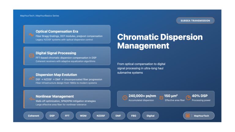
Chromatic Dispersion Management in Subsea Systems Subsea Transmission Technology Chromatic Dispersion Management in Subsea Systems From Optical Compensation to Digital...
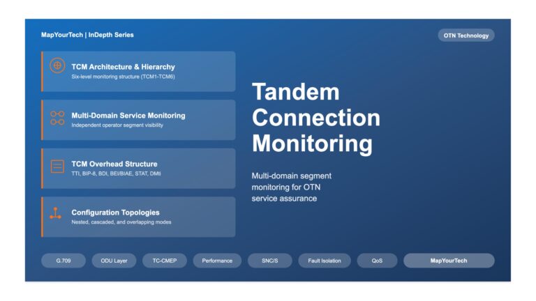
Tandem Connection Monitoring in OTN Networks | MapYourTech Tandem Connection Monitoring in Optical Transport Networks Comprehensive guide to multi-domain service...
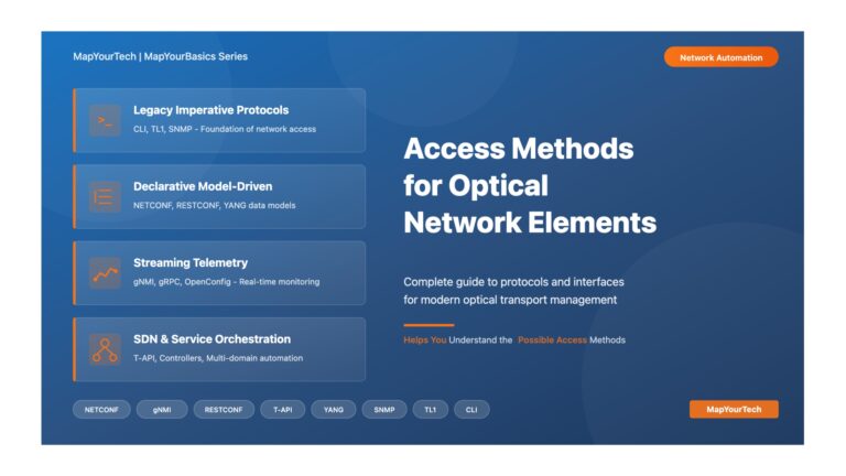
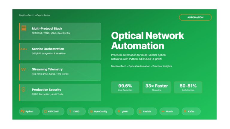
Access Methods for Optical Network Elements | MapYourTech Optical Network Automation Access Methods for Optical Network Elements A Comprehensive Guide...