Inter-DC vs Intra-DC for Optical Professionals: Complete Guide Inter-DC vs Intra-DC for Optical Professionals A comprehensive guide to understanding data...
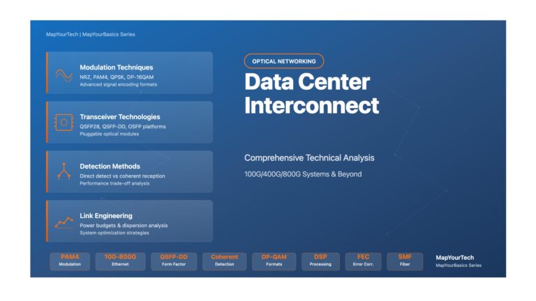
Data Center Interconnect: Comprehensive Technical Analysis Data Center Interconnect Technology A Comprehensive Technical Analysis of 100G/400G/800G Systems, PAM4 Modulation, and...
Advanced Deep Dive: Raman Amplifier – Everything About It Advanced Deep Dive: Raman Amplifiers Comprehensive Expert-Level Analysis of Stimulated Raman...