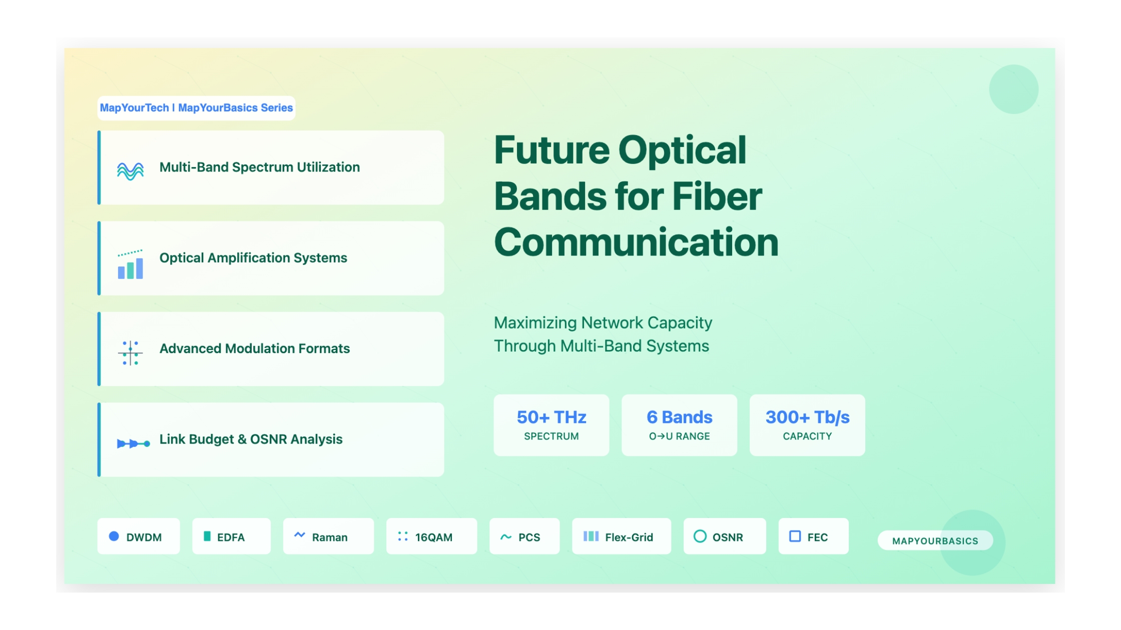

Future Optical Bands for Communication to Increase Fiber Capacity
A Comprehensive Technical Guide to Multi-Band Optical Transmission Systems
Fundamentals & Core Concepts
What is Multi-Band Optical Communication?
Multi-band optical communication represents the strategic expansion of wavelength division multiplexing (WDM) systems beyond the traditional C-band (1530-1565 nm) and L-band (1565-1625 nm) into additional spectral windows including the O-band (1260-1360 nm), E-band (1360-1460 nm), S-band (1460-1530 nm), and U-band (1625-1675 nm). This approach unlocks the full low-loss transmission window of modern optical fibers, spanning over 50 THz of spectrum from approximately 180 THz to 230 THz.
Why Do We Need Extended Optical Bands?
The Capacity Crunch: The global demand for data transmission capacity is experiencing unprecedented growth, driven by 5G networks, cloud computing, virtual reality, ultra-high-definition video, and the Internet of Things (IoT). Traditional C+L band systems are approaching their fundamental spectral efficiency limits as defined by Shannon's theorem.
Physical Origins: The viability of different optical bands stems from the intrinsic properties of silica-based optical fibers. Rayleigh scattering, which scales proportionally to λ⁻⁴, dictates that shorter wavelengths experience higher attenuation. Modern G.652.D fibers achieve minimum loss of ≤0.18 dB/km at 1550 nm (C-band), with the attenuation spectrum defining which wavelength regions are practical for transmission.
When Does Multi-Band Matter?
- Capacity Exhaustion: When C+L bands reach maximum utilization and additional capacity is required on existing fiber infrastructure
- Long-Haul Networks: For submarine and ultra-long-haul systems where maximizing fiber capacity justifies higher equipment costs
- Metropolitan Networks: When fiber scarcity or lease costs make multi-band operation economically attractive
- Future-Proofing: When designing new networks to support decades of traffic growth
Why Is It Important?
The significance of multi-band optical transmission extends beyond mere capacity scaling. It represents a fundamental shift in how we approach optical network design, addressing economic, technical, and strategic imperatives:
- Economic Efficiency: Maximizes return on fiber infrastructure investment by utilizing existing dark fiber more intensively
- Environmental Sustainability: Reduces the need for new fiber deployments, minimizing environmental impact and construction costs
- Scalability: Provides a clear path for capacity growth for 10-20 years without requiring new fiber installations
- Competitive Advantage: Enables service providers to offer higher bandwidth services and meet customer demands
Mathematical Framework
Shannon-Hartley Theorem for Optical Channels
C = B × log₂(1 + SNR)
Where:
- C = Channel capacity (bits per second)
- B = Bandwidth (Hertz)
- SNR = Signal-to-Noise Ratio (dimensionless)
Key Implication: Each 1-bit/symbol increase in spectral efficiency requires approximately a +3 dB increase in SNR, which typically halves the achievable transmission distance.
Optical Signal-to-Noise Ratio (OSNR)
SNRpol = (2 × Bref) / (p × Rs) × OSNR
Where:
- SNRpol = Per-polarization electrical SNR
- Bref = Reference optical bandwidth (typically 12.5 GHz for 0.1 nm)
- Rs = Symbol rate (GBaud)
- p = 1 for non-PDM signals, 2 for PDM signals
- OSNR = Optical Signal-to-Noise Ratio
Total System Capacity Calculation
Ctotal = N × Rs × m × ηFEC
Where:
- N = Number of WDM channels
- Rs = Symbol rate per channel (GBaud)
- m = Bits per symbol (log₂ of modulation order, e.g., 4 for 16QAM)
- ηFEC = FEC efficiency (typically 0.80-0.93)
Example Calculation: For a C-band system with 96 channels, 32 GBaud symbol rate, 16QAM modulation (4 bits/symbol), and 20% FEC overhead (η = 0.833):
Ctotal = 96 × 32 × 4 × 0.833 = 10.22 Tb/s
Spectral Efficiency
SE = Ctotal / Btotal
Where:
- SE = Spectral Efficiency (bits/s/Hz)
- Ctotal = Total system capacity (bits/s)
- Btotal = Total optical bandwidth (Hz)
Practical Values: Modern systems achieve 3-6 bits/s/Hz with QPSK to 16QAM, approaching Shannon limits of 8-10 bits/s/Hz with advanced techniques like probabilistic constellation shaping.
Optical Band Classification & Components
ITU-T Defined Optical Bands
| Band | Wavelength Range | Frequency Range | Typical Loss | Primary Applications |
|---|---|---|---|---|
| O-Band (Original) | 1260-1360 nm | 220-238 THz | ≤0.35 dB/km | PONs, Data Centers, Short-reach |
| E-Band (Extended) | 1360-1460 nm | 205-220 THz | ≤0.35 dB/km (ZWP) | Capacity expansion (G.652.D fiber) |
| S-Band (Short) | 1460-1530 nm | 196-205 THz | ≤0.25 dB/km | PON, DWDM expansion |
| C-Band (Conventional) | 1530-1565 nm | 191-196 THz | ≤0.18 dB/km | Long-haul, Metro, Submarine |
| L-Band (Long) | 1565-1625 nm | 184-191 THz | ≤0.20 dB/km | Capacity doubling with C-band |
| U-Band (Ultralong) | 1625-1675 nm | 179-184 THz | ≤0.25 dB/km | Future capacity, monitoring |
Super C and Super L Band Extensions
Super L-Band: Extends conventional L-band from 4.8 THz to 5.5 THz (approximately 1575-1622 nm), adding 0.7 THz (14.5% increase)
These extensions maximize capacity on existing infrastructure before deploying full multi-band systems, leveraging mature EDFA technology with component upgrades.
Amplifier Technology Comparison
| Technology | Operating Bands | Typical Gain | Noise Figure | Key Advantages | Challenges |
|---|---|---|---|---|---|
| EDFA | C, L | 20-30 dB | 4-6 dB | Mature, cost-effective, high power | Limited to C/L bands |
| Raman (Distributed) | All bands | 10-20 dB | <0 dB (effective) | Flexible, improves OSNR | High pump power, complex control |
| TDFA | S, U | 20-25 dB | 5-8 dB | S-band coverage | Non-silica fiber, complex pumping |
| BDFA | O, E, S, U | 20-30 dB | 4-6 dB | Ultra-wideband potential | Developing technology |
| SOA | O, E, S, C, L | 20-30 dB | 5-8 dB | Compact, integrable | Crosstalk, polarization sensitivity |
| PDFA | O (1280-1330 nm) | >24 dB | 6-7 dB | Flat gain, low distortion | Requires fluoride fiber |
System Effects & Performance Impacts
Fiber Attenuation Characteristics
The fundamental limitation of optical transmission is fiber attenuation, which varies significantly across different spectral bands due to Rayleigh scattering (λ⁻⁴ dependence) and material absorption:
- C-Band (1550 nm): 0.18 dB/km - enables 4000+ km transmission with amplification
- O-Band (1310 nm): 0.35 dB/km - approximately 50% higher loss limits long-haul applications
- S-Band (1490 nm): 0.25 dB/km - moderate loss, viable for extended networks
- U-Band (1650 nm): 0.25 dB/km - benefits from ISRS gain from shorter wavelengths
Nonlinear Impairments in Wideband Systems
Inter-Channel Stimulated Raman Scattering (ISRS)
ISRS causes energy transfer from shorter to longer wavelengths across the WDM spectrum, creating power tilt. In a 50 THz wideband system, ISRS can induce 10-15 dB of power variation between O-band and U-band channels if uncompensated.
Four-Wave Mixing (FWM)
FWM is particularly problematic in O-band due to low chromatic dispersion. When channels at frequencies f₁, f₂, and f₃ mix, new frequency components are generated at f₄ = f₁ + f₂ - f₃, causing interference.
Cross-Phase Modulation (XPM)
XPM causes phase shifts in one channel due to intensity variations in neighboring channels, degrading signal quality in dense WDM systems.
OSNR Requirements by Modulation Format
| Modulation Format | Bits/Symbol (PDM) | Typical OSNR Required | Spectral Efficiency | Relative Reach |
|---|---|---|---|---|
| PM-QPSK | 4 | 10-12 dB | 2.0 bits/s/Hz | 100% (baseline) |
| PM-8QAM | 6 | 14-16 dB | 3.0 bits/s/Hz | ~70% |
| PM-16QAM | 8 | 17-19 dB | 4.0 bits/s/Hz | ~50% |
| PM-32QAM | 10 | 20-22 dB | 5.0 bits/s/Hz | ~35% |
| PM-64QAM | 12 | 23-25 dB | 6.0 bits/s/Hz | ~25% |
| PM-256QAM | 16 | 29-32 dB | 8.0 bits/s/Hz | ~12% |
Advanced Techniques & Solutions
Probabilistic Constellation Shaping (PCS)
PCS represents a paradigm shift in optical transmission by optimizing the probability distribution of transmitted symbols rather than just constellation geometry. Lower-energy constellation points are transmitted more frequently than higher-energy points, approximating a Gaussian distribution optimal for AWGN channels.
- Shaping Gain: 0.5-1.5 dB OSNR improvement at target BER
- Fine-Grained Rate Adaptation: Continuous rate adjustment matching channel conditions
- Extended Reach: 15-30% transmission distance increase for same modulation format
- Flexibility: Dynamic optimization for varying network conditions
Nyquist Pulse Shaping and Nyquist-WDM
Nyquist pulse shaping uses pulses satisfying Nyquist's first criterion for zero inter-symbol interference (ISI). Root-raised-cosine (RRC) filters with small roll-off factors (α = 0.01-0.1) confine signal energy within the Nyquist bandwidth, enabling channel spacing approaching the symbol rate (Δf ≈ Rs).
Spectral Efficiency: Nyquist-WDM eliminates guard bands, achieving theoretical maximum spectrum utilization. With 32 GBaud symbol rate and α = 0.05, channel spacing can be reduced to ~33 GHz, compared to 50 GHz for traditional systems.
Advanced Forward Error Correction (FEC)
| FEC Type | Coding Gain | Overhead | Latency | Applications |
|---|---|---|---|---|
| Hard-Decision FEC | 6-7 dB | 7% | Low | Short-reach, cost-sensitive |
| Soft-Decision LDPC | 10-11 dB | 20% | Medium | Metro, regional |
| Concatenated FEC | 11-12 dB | 25% | High | Long-haul, submarine |
| Polar Codes | 12+ dB | 20-27% | Medium-High | Ultra-long-haul, future systems |
Flexible Grid DWDM (Flex-Grid)
ITU-T G.694.1 flex-grid defines frequency slots with 12.5 GHz minimum granularity, allowing dynamic spectrum allocation matched to signal requirements. Traditional 50 GHz fixed grids waste spectrum when signals require less bandwidth or cannot accommodate wide signals efficiently.
- Spectrum Efficiency: 20-40% improvement through right-sizing channels
- Mixed Bit Rates: Accommodates 100G, 200G, 400G, 1T signals on same fiber
- Future-Proof: Supports evolving modulation formats and symbol rates
- Elastic Optical Networks: Enables software-defined networking (SDN) control
Gain Equalization and Power Management
Wideband systems require sophisticated gain flattening to ensure uniform channel performance across 50+ THz spectrum:
Static Gain Flattening Filters (GFF): Passive filters with inverse EDFA gain profile, typically achieving ±0.5 dB flatness over 35 nm
Dynamic Gain Equalizers (DGE): Active devices using acousto-optic tunable filters (AOTF) or integrated photonics for real-time gain adjustment, compensating for channel loading variations and amplifier aging
Multi-Pump Raman Optimization: 6-8 pump wavelengths at different powers shape composite Raman gain profile across C+L or wider bands
Design Guidelines & Methodology
Multi-Band System Design Process
Step 1: Requirements Analysis
- Define target capacity and growth projections (5-10 year horizon)
- Determine maximum transmission distance and amplifier spacing
- Establish acceptable bit error rate (typical: 10⁻¹⁵ post-FEC)
- Identify fiber type in deployment (G.652.D, G.654.E, G.655, legacy)
- Assess existing amplifier infrastructure and upgrade feasibility
Step 2: Band Selection Strategy
- Phase 1: Maximize C-band utilization (80-96 channels at 50 GHz spacing)
- Phase 2: Add L-band (double capacity to ~160-192 channels)
- Phase 3: Consider Super C or Super L extensions (add 20-30% more channels)
- Phase 4: Evaluate S-band or U-band for ultra-high capacity scenarios
- Phase 5: Full multi-band (O+E+S+C+L+U) for maximum density
Step 3: Link Budget Calculation
PRX = PTX + Gamp - Lfiber - Lconnector - Lcomponent - Msystem
Component Breakdown:
- PTX: Transmitter launch power (typically +2 to +5 dBm per channel)
- Gamp: Total amplifier gain (compensates span loss)
- Lfiber: Fiber attenuation × distance (α × L)
- Lconnector: Connector losses (~0.3 dB per connector pair)
- Lcomponent: WSS, MUX/DEMUX, OADM losses (3-8 dB per ROADM node)
- Msystem: System margin for aging, repairs (3-5 dB typical)
Example: For 80 km span with 0.20 dB/km fiber at 1550 nm:
Lfiber = 0.20 × 80 = 16 dB
If PTX = +3 dBm, target PRX = -15 dBm, with 2 dB component loss and 3 dB margin:
Required Gamp = -15 - 3 + 16 + 2 + 3 = 3 dB per span
Step 4: OSNR Budget Analysis
Calculate end-of-life OSNR considering ASE noise accumulation across multiple amplifier spans:
OSNR after N spans:
OSNRN = Psignal / (N × PASE)
Where PASE ≈ 2 × nsp × h × ν × Bref × (G - 1)
Step 5: Modulation Format Selection
| Available OSNR | Recommended Format | Expected SE | Typical Use Case |
|---|---|---|---|
| <12 dB | PM-QPSK | 2.0 b/s/Hz | Ultra-long-haul (>3000 km) |
| 12-16 dB | PM-8QAM | 3.0 b/s/Hz | Long-haul (1500-3000 km) |
| 16-20 dB | PM-16QAM | 4.0 b/s/Hz | Regional (500-1500 km) |
| 20-25 dB | PM-32/64QAM | 5.0-6.0 b/s/Hz | Metro (100-500 km) |
| >25 dB | PM-64/256QAM | 6.0-8.0 b/s/Hz | Short-reach (<100 km) |
Design Checklist
- ✓ Verify fiber type supports target bands (check E-band water peak for legacy fiber)
- ✓ Confirm amplifier bandwidth coverage across all deployed bands
- ✓ Design gain equalization for ±1 dB flatness across full spectrum
- ✓ Account for ISRS power tilt in wideband systems (>15 THz)
- ✓ Validate WSS and MUX/DEMUX components support required bandwidth
- ✓ Plan for FEC overhead in capacity calculations (15-25% typical)
- ✓ Include system margin for component aging and repairs (3-5 dB)
- ✓ Consider nonlinear impairments: adjust launch power per channel
- ✓ Implement chromatic dispersion compensation strategy
- ✓ Verify polarization mode dispersion (PMD) within acceptable limits
Common Pitfalls to Avoid
- Underestimating Component Losses: ROADM nodes with multiple WSS can add 6-10 dB per node
- Ignoring ISRS Effects: Can create 10+ dB power tilt across 50 THz requiring active management
- Inadequate Gain Flattening: Channel OSNR variation leads to some channels failing while others over-perform
- FEC Overhead Neglect: 20% FEC reduces 100G to 80G net capacity
- Legacy Fiber Assumptions: Old fiber may have high E-band loss due to water peak
- Amplifier Compatibility: Not all "C-band" EDFAs support full extended C-band (1529-1567 nm)
Interactive Simulators & Tools
Practical Applications & Case Studies
Real-World Deployment Scenarios
Scenario 1: Metropolitan Area Network Upgrade
- Existing Infrastructure: G.652.D fiber, 96-channel C-band DWDM at 50 GHz spacing
- Current Capacity: 9.6 Tb/s (100G per channel, PM-QPSK)
- Demand Growth: 40% year-over-year requiring 25+ Tb/s within 3 years
- Typical Span: 40-60 km, 3-5 ROADM nodes
- Added L-band (96 channels) for immediate capacity doubling
- Upgraded transceivers to 200G PM-16QAM for newer routes
- Deployed hybrid EDFA-Raman amplifiers for improved OSNR
- Implemented flex-grid for mixed 100G/200G/400G services
Scenario 2: Submarine Cable System
- Distance: 8,000 km with amplifier spacing every 50 km
- Fiber Type: G.654.E with 0.17 dB/km at 1550 nm
- Target Capacity: 300+ Tb/s to support cloud provider demand
- Lifespan: 25 years with multiple capacity upgrades
- Deployed 24-fiber pairs with wideband amplification
- S-band: 50 channels (TDFA + Raman)
- C-band: 96 channels (EDFA + distributed Raman)
- L-band: 96 channels (EDFA + distributed Raman)
- U-band: 40 channels (Raman only with ISRS gain)
- Adaptive modulation: PM-QPSK for longest spans, PM-16QAM for shorter segments
- Advanced FEC with 25% overhead for maximum reach
Scenario 3: Data Center Interconnect (DCI)
- Distance: 80-300 km between major facilities
- Capacity Need: 100+ Tb/s for east-west traffic, AI/ML workloads
- Latency Requirement: <5 ms round-trip
- Growth Rate: Doubling every 18-24 months
- 120 channels per band (240 total) at 37.5 GHz spacing using flex-grid
- 800G wavelengths using PM-64QAM with probabilistic constellation shaping
- Ultra-low-loss G.654.E fiber (0.16 dB/km) minimizing amplifier count
- Coherent pluggable optics (QSFP-DD, OSFP form factors)
- Soft-decision FEC with 15% overhead optimized for high OSNR
Troubleshooting Guide
| Symptom | Probable Cause | Diagnostic Steps | Remediation |
|---|---|---|---|
| OSNR degradation at longer wavelengths | ISRS power tilt accumulating across spans | Measure per-channel power at multiple points; verify >5 dB tilt | Implement tilt compensation via DGE or multi-pump Raman optimization |
| High BER in E-band channels only | Legacy fiber with water peak around 1383 nm | Check fiber specification; measure loss at 1383 nm (should be <0.4 dB/km) | Replace with G.652.D fiber or avoid E-band deployment |
| Intermittent signal loss | Amplifier ASE transients from channel add/drop | Monitor amplifier gain during provisioning events | Enable fast link control and per-channel power management |
| Poor S-band performance | Insufficient TDFA gain or high noise figure | Verify TDFA pump power, check NF (>7 dB problematic) | Upgrade to hybrid TDFA+Raman or optimize pump wavelengths |
| Spectral holes in flex-grid | Improper frequency slot allocation or WSS filtering | Analyze spectrum with OSA; verify slot boundaries | Reconfigure controller for proper 12.5 GHz grid alignment |
| Nonlinear crosstalk in O-band | Four-wave mixing due to low dispersion | Calculate FWM efficiency; check if channels at f1+f2-f3 | Reduce launch power, use unequal channel spacing, or add dispersion |
Quick Reference: Band Selection Matrix
| Application | Distance | Capacity | Recommended Bands | Rationale |
|---|---|---|---|---|
| Data Center | <10 km | High | O-band single channel | Zero dispersion, low cost, no amplification |
| Metro Access | 10-80 km | Medium | C-band DWDM | Mature ecosystem, EDFA availability |
| Metro Core | 80-300 km | High | C+L bands | Double capacity, proven technology |
| Regional | 300-1000 km | Very High | C+L or S+C+L | Balance capacity and amplifier maturity |
| Long-Haul | 1000-3000 km | Ultra High | S+C+L+U | Maximum capacity justifies hybrid amplifiers |
| Submarine | >3000 km | Extreme | All bands (O through U) | Fiber scarcity justifies maximum utilization |
Professional Recommendations
- Start Conservative: Begin with well-proven C+L before venturing into extended bands
- Plan for Growth: Design amplifier infrastructure to support future band additions
- Monitor Proactively: Implement comprehensive OSA and OSNR monitoring across all bands
- Staged Upgrades: Upgrade transceivers before adding new bands to maximize existing spectrum
- Vendor Alignment: Ensure consistent multi-vendor interoperability for components
- Test Thoroughly: Validate performance under full load with worst-case channel plans
- Document Everything: Maintain detailed as-built records of per-band configurations
- Training Investment: Ensure operations teams understand multi-band system behaviors
- Automation: Deploy SDN controllers for dynamic spectrum and routing management
- Future-Proof: Select equipment supporting software upgrades to new modulation formats
Key Takeaways
- 1. Multi-Band Strategy: Expanding beyond C+L bands unlocks 50+ THz of spectrum, potentially increasing fiber capacity from 50 Tb/s to over 300 Tb/s per fiber.
- 2. Band Characteristics: O-band (1260-1360 nm) offers zero dispersion for short reach; E-band requires zero-water-peak fiber; S-band needs TDFA/BDFA; C-band and L-band remain most mature; U-band benefits from ISRS gain.
- 3. Amplifier Diversity: No single amplifier covers all bands—EDFAs for C/L, TDFAs for S, Raman for flexibility, BDFAs/SOAs for emerging bands. Hybrid approaches essential for ultra-wideband systems.
- 4. Shannon Limit Trade-offs: Each 3 dB SNR increase enables 1 bit/symbol higher modulation but halves transmission reach. Current systems operate within 1-2 dB of theoretical limits.
- 5. ISRS Management: Wideband systems experience 10-15 dB power tilt across 50 THz requiring active gain equalization and multi-pump Raman optimization.
- 6. Spectral Efficiency: Probabilistic constellation shaping provides 0.5-1.5 dB shaping gain; Nyquist-WDM eliminates guard bands; flex-grid enables 20-40% better spectrum utilization.
- 7. Modulation Selection: PM-QPSK for ultra-long-haul (>3000 km), PM-16QAM for regional (500-1500 km), PM-64QAM+ for metro (<500 km) based on OSNR availability.
- 8. Link Budget Discipline: Account for fiber loss (0.18-0.35 dB/km by band), component losses (6-10 dB per ROADM node), FEC overhead (15-25%), and system margin (3-5 dB).
- 9. Phased Deployment: Maximize C-band first, add L-band for doubling, consider Super C/L extensions (+20-30%), then S or U-band for extreme capacity, finally full O-through-U for submarine.
- 10. Economic Reality: Multi-band systems cost 30-60% more than C-band alone but avoid fiber installation costs ($50K-$200K per km), making them economically viable when fiber is scarce or capacity exhausted.
Developed by MapYourTech Team for educational purposes
Note: This guide is based on industry standards, best practices, and real-world implementation experiences. Specific implementations may vary based on equipment vendors, network topology, and regulatory requirements. Always consult with qualified network engineers and follow vendor documentation for actual deployments.

Optical Communications & Network Automation Expert | Author of 3 Books for Optical Engineers | Founder, MapYourTech
Optical networking engineer with nearly two decades of experience across DWDM, OTN, coherent optics, submarine systems, and cloud infrastructure. Founder of MapYourTech. Read full bio →
Follow on LinkedInRelated Articles on MapYourTech