Passive Optical Networks (PON)
Executive Summary
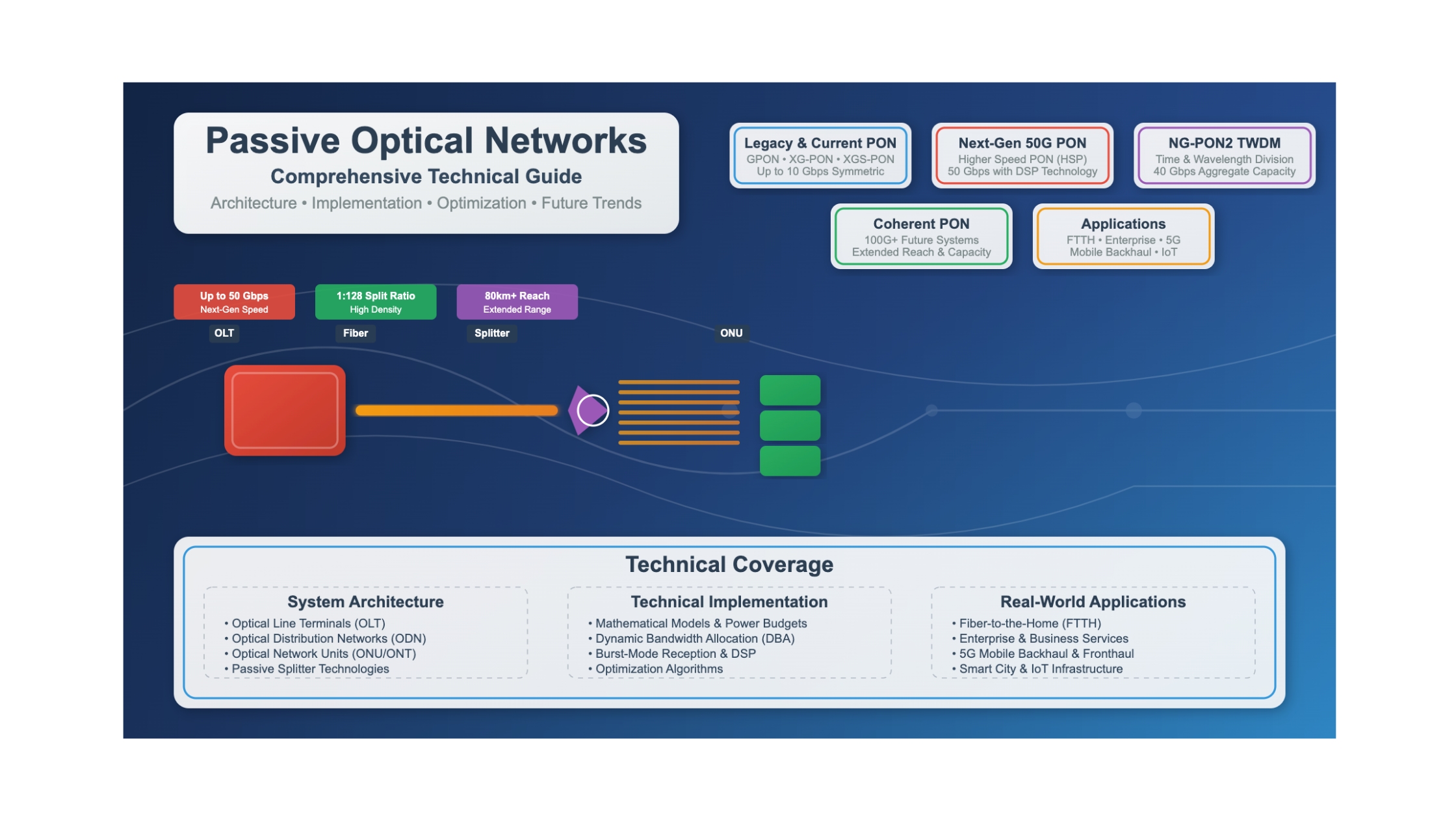
Passive Optical Networks (PON) represent the cornerstone of modern fiber-to-the-home (FTTH) infrastructure, providing cost-effective, scalable, and high-performance broadband access to millions of users worldwide. This comprehensive technical analysis examines the complete ecosystem of PON technologies, from foundational principles to the latest 2025 developments in 50G-PON and emerging 100G Coherent PON systems.
As of 2025, the global PON market has reached $17.66 billion and is projected to grow to $44.46 billion by 2032, driven by increasing bandwidth demands for 8K video streaming, virtual reality applications, cloud computing, and 5G mobile backhaul requirements. The technology landscape has significantly evolved with the commercial introduction of 50G-PON systems and active development of 100G Coherent PON solutions.
Critical Implications for 2025 and Beyond:
- Technology Transition: 50G-PON systems are entering commercial deployment phase with dual-rate capabilities (50G/25G and 50G/50G)
- Market Disruption: Coherent PON technologies promise 100G+ speeds with superior reach (80km vs 25km traditional limit)
- Economic Impact: Cost differential between 50G intensity modulation and 100G coherent solutions narrowing significantly
- Infrastructure Optimization: Backward compatibility ensures seamless coexistence with legacy GPON and XGS-PON deployments
- Application Expansion: PON adoption extending beyond residential to enterprise, data center interconnects, and 5G transport networks
This analysis provides network architects, telecommunications engineers, and technology decision-makers with the comprehensive understanding necessary to navigate the rapidly evolving PON landscape and make informed infrastructure investment decisions.
Historical Context & Foundational Principles
Evolution Timeline: From BPON to 100G Coherent PON
BPON Era (Broadband PON)
ITU-T G.983 standard introduced the first passive optical network architecture with 155/622 Mbps rates. Established fundamental point-to-multipoint topology using passive optical splitters.
GPON & EPON Deployment
GPON (ITU-T G.984) delivering 2.488 Gbps downstream, 1.244 Gbps upstream. IEEE 802.3ah EPON standardized with symmetric 1.25 Gbps. Mass FTTH deployments begin globally.
10G PON Generation
XG-PON (G.987) and XGS-PON (G.9807) introduced 10 Gbps capabilities. 10G-EPON (802.3av) standardized. First wavelength division multiplexing implementations.
NG-PON2 & TWDM
ITU-T G.989 series introduces Time and Wavelength Division Multiplexed PON with 40 Gbps aggregate capacity using four 10G wavelength channels. Point-to-point WDM overlay capability.
Higher Speed PON (HSP)
ITU-T G.9804 series approved for 50G-PON. Digital signal processing introduced. IEEE 802.3ca 25G/50G-EPON standardized. First field trials demonstrate commercial viability.
Coherent PON Era
100G+ Coherent PON systems under development. Extended reach up to 80km. AI-enhanced network management. Unified platform for residential, enterprise, and mobile backhaul services.
Foundational Architecture Principles
Core Operating Principles
PON architecture fundamentally relies on four key principles that distinguish it from active optical networking approaches:
1. Passive Optical Distribution
The optical distribution network (ODN) contains no active electronic components between the OLT and ONUs. Passive optical splitters divide the optical signal power among multiple distribution paths, typically supporting split ratios from 1:8 to 1:128. This passive nature significantly reduces operational complexity, power consumption, and maintenance requirements while improving system reliability.
2. Wavelength Division for Bidirectional Communication
PON systems employ wavelength division multiplexing (WDM) to enable simultaneous bidirectional communication over a single fiber. Downstream signals typically operate at longer wavelengths (1480-1500nm for GPON, 1575-1580nm for XG-PON) while upstream signals use shorter wavelengths (1260-1360nm range). This wavelength separation eliminates the need for separate upstream and downstream fibers.
Ptx,OLT - Prx,ONU = Lfiber + Lsplitter + Lconnector + Mmargin
Where:
Ptx,OLT = OLT transmit power (dBm)
Prx,ONU = ONU receiver sensitivity (dBm)
Lsplitter = 10 × log10(N) dB for 1:N split ratio
Mmargin = System margin (typically 3-5 dB)
3. Time Division Multiple Access (TDMA)
Upstream communication utilizes TDMA to prevent collision between signals from multiple ONUs. The OLT coordinates transmission schedules through Dynamic Bandwidth Allocation (DBA) algorithms, ensuring efficient bandwidth utilization while maintaining Quality of Service (QoS) requirements for different traffic classes.
4. Burst-Mode Operation
ONUs transmit data in synchronized bursts during allocated time slots. This requires sophisticated burst-mode receivers at the OLT capable of rapidly adjusting gain and threshold levels between bursts from different ONUs operating at varying optical power levels and wavelengths.
Market Evolution and Current Landscape (2025)
The global PON market has experienced unprecedented growth, reaching $17.66 billion in 2025 with projections indicating expansion to $44.46 billion by 2032. This growth trajectory reflects several converging factors:
| Market Segment | 2024 Market Share | Growth Driver | Technology Preference |
|---|---|---|---|
| Residential Broadband | 44.2% (GPON dominant) | 8K video, cloud gaming, smart homes | Transition to XGS-PON, early 25G/50G adoption |
| Enterprise Services | 28.7% | Cloud computing, remote work, video conferencing | XGS-PON, increasing 25G/50G deployment |
| Mobile Backhaul | 15.8% (fastest growing) | 5G network densification, low-latency requirements | XGS-PON, 50G-PON for small cell aggregation |
| Data Center Interconnect | 11.3% | Edge computing, content distribution | NG-PON2, emerging 100G Coherent PON |
Regional deployment patterns show significant variation, with Asia-Pacific leading global adoption at 49.13% market share, driven primarily by China's aggressive fiber infrastructure investments and the "Digital Village" initiative targeting rural connectivity. North America maintains substantial market presence supported by federal funding programs including the Rural Digital Opportunity Fund (RDOF) and Infrastructure Investment and Jobs Act (IIJA).
Technical Architecture & System Design
Comprehensive Component Architecture
Modern PON systems comprise three fundamental architectural domains, each with distinct technical requirements and performance characteristics. Understanding the intricate relationships between these components is essential for optimal system design and deployment planning.
Optical Line Terminal (OLT) Architecture
The OLT serves as the service provider endpoint, performing critical functions including optical-electrical signal conversion, traffic aggregation, bandwidth management, and service provisioning. Advanced OLT designs incorporate multiple line cards (optical subscriber units) to support various PON technologies simultaneously.
Advanced OLT Features in 2025 Systems
Contemporary OLT designs incorporate several advanced capabilities to support next-generation PON services:
- Multi-Generation Coexistence: Single chassis supporting GPON, XGS-PON, 50G-PON, and NG-PON2 line cards simultaneously
- AI-Enhanced DBA: Machine learning algorithms optimize bandwidth allocation based on traffic patterns and QoS requirements
- Coherent DSP Integration: Digital signal processing capabilities for 100G+ coherent PON applications
- Network Function Virtualization: Software-defined functionality enabling rapid service deployment and management
- Advanced Security: Hardware-based encryption, secure boot mechanisms, and automated threat detection
Optical Network Unit (ONU/ONT) Evolution
ONUs have evolved from simple optical-electrical converters to sophisticated multi-service platforms supporting residential, business, and mobile backhaul applications. Modern ONUs incorporate advanced features including tunable transceivers, digital signal processing, and AI-enhanced edge computing capabilities.
| ONU Generation | Key Technologies | Typical Applications | Performance Metrics |
|---|---|---|---|
| GPON ONU | Fixed wavelength, burst-mode upstream | Residential broadband, basic business | 2.5G/1.25G, 28 dB budget |
| XGS-PON ONU | Enhanced receivers, improved sensitivity | High-speed residential, SMB/SME | 10G/10G symmetric, 29-35 dB budget |
| NG-PON2 ONU | Tunable transceivers, WDM capability | Enterprise, data center, mobile backhaul | 10G per wavelength, 4×10G aggregate |
| 50G-PON ONU | DSP, advanced modulation, dual-rate | Ultra-broadband, 5G transport, enterprise | 50G/25G or 50G/50G, extended reach |
| Coherent PON ONU | Coherent detection, adaptive modulation | 100G+ services, long-reach applications | 100G+ symmetric, 39+ dB budget |
Srx = Pmin + NF + 10×log10(B) + SNRreq - Gcoding
Where:
Pmin = Minimum detectable power (-174 dBm/Hz at room temperature)
NF = Noise figure of receiver (dB)
B = Signal bandwidth (Hz)
SNRreq = Required signal-to-noise ratio for target BER
Gcoding = Forward error correction coding gain (dB)
Core Concepts & Terminology
Understanding PON technology requires mastery of specialized terminology and fundamental concepts that govern optical network behavior, signal processing, and system performance. This section provides comprehensive definitions and conceptual models essential for PON design and deployment.
Fundamental PON Terminology
Dynamic Bandwidth Allocation (DBA)
Modern DBA implementations use machine learning to predict traffic patterns and optimize bandwidth utilization. Advanced algorithms consider Service Level Agreements (SLAs), traffic priority classes, and real-time network conditions.
Optical Distribution Network (ODN)
ODN design critically impacts system performance, supporting various topologies including tree, bus, and ring configurations. Power budget calculations determine maximum reach and split ratios.
Time and Wavelength Division Multiplexing (TWDM)
TWDM-PON architecture enables multiple wavelength channels each supporting independent TDM-PON domains, significantly expanding system capacity while maintaining backward compatibility.
Burst-Mode Reception
Critical for TDMA operation, requiring fast automatic gain control (AGC), clock and data recovery (CDR), and threshold adjustment within microsecond timeframes.
Forward Error Correction (FEC)
Modern PON systems employ Reed-Solomon, BCH, or LDPC codes. 50G-PON introduces flexible FEC options optimizing performance for different deployment scenarios.
Coherent Detection
Enables superior sensitivity compared to direct detection, supporting 100G+ PON systems with extended reach capabilities up to 80km.
Advanced Conceptual Models
PON Protocol Stack Architecture
Wavelength Allocation and Coexistence Models
Modern PON deployments require sophisticated wavelength planning to enable coexistence of multiple PON generations on the same ODN infrastructure. The wavelength allocation strategy significantly impacts system performance, upgrade paths, and operational complexity.
| PON Technology | Downstream Wavelength | Upstream Wavelength | Coexistence Capability | Special Requirements |
|---|---|---|---|---|
| GPON | 1480-1500 nm | 1260-1360 nm | Foundation technology | RF video overlay at 1550-1560 nm |
| XGS-PON | 1575-1580 nm | 1260-1280 nm | GPON + XGS-PON | Enhanced FEC, higher launch power |
| NG-PON2 TWDM | 1596-1603 nm (4×λ) | 1524-1544 nm (4×λ) | Triple coexistence possible | Tunable transceivers, WDM filters |
| 50G-PON | 1342±2 nm | 1286±2 nm | GPON + XGS + 50G | DSP, flexible FEC, dual-rate |
| 100G Coherent PON | C/L-band (1530-1625 nm) | C/L-band (1530-1625 nm) | Overlay with all generations | Coherent transceivers, advanced DSP |
Mathematical Models & Performance Analysis
Fundamental Optical Power Budget Modeling
Accurate power budget calculations form the foundation of PON system design, determining maximum reach, split ratios, and performance margins. The comprehensive power budget model accounts for all optical losses and system impairments.
Complete Power Budget Equation:
Ptx,OLT - Prx,ONU ≥ Lfiber + Lsplitter + Lconnector + Lsplice + Laging + MsystemDetailed Component Analysis:
• Lfiber = α × d (α = 0.35-0.4 dB/km for 1310nm, 0.2-0.25 dB/km for 1550nm)
• Lsplitter = 10 × log10(N) + Lexcess (N = split ratio, Lexcess ≈ 1-3 dB)
• Lconnector = 0.5 dB per connection
• Lsplice = 0.1 dB per fusion splice
• Laging = 1-2 dB (component degradation over 20+ years)
• Msystem = 3-5 dB (temperature variations, penalties, margin)
Advanced Split Ratio Calculations
Split ratio selection critically impacts both system economics and performance. Higher split ratios reduce per-customer fiber infrastructure costs but impose stricter optical budget requirements.
1:32 Split Configuration
Optical Loss: 15.1 dB
Reach: Up to 20 km
Customer Density: Medium
Applications: Suburban/rural FTTH
1:64 Split Configuration
Optical Loss: 18.1 dB
Reach: Up to 15 km
Customer Density: High
Applications: Urban FTTH, MDU
1:128 Split Configuration
Optical Loss: 21.1 dB
Reach: Up to 10 km
Customer Density: Very high
Applications: Dense urban, enterprise
Signal Quality and Performance Metrics
Bit Error Rate (BER) Analysis
BER performance determines system reliability and directly impacts customer Quality of Experience (QoE). Modern PON systems target BER ≤ 10⁻¹² for error-free operation after FEC.
BER = (1/2) × erfc(Q/√2)
Where Q-factor = (I₁ - I₀) / (σ₁ + σ₀)
I₁, I₀ = Signal levels for '1' and '0' bits
σ₁, σ₀ = Noise standard deviations
For OSNR-limited systems:
Q = √(OSNR × Rs / (2 × Bopt))
Rs = Symbol rate, Bopt = Optical bandwidth
Forward Error Correction (FEC) Performance
FEC coding provides significant coding gain, improving effective receiver sensitivity. Different FEC schemes offer varying complexity-performance trade-offs.
| FEC Type | Code Rate | Coding Gain (dB) | Correctable Errors | PON Applications |
|---|---|---|---|---|
| Reed-Solomon (255,239) | 0.937 | 5.9 | 8 symbols | GPON, XG-PON |
| BCH (2040, 1952) | 0.957 | 6.2 | 44 bits | XGS-PON |
| LDPC (2048, 1723) | 0.841 | 8.5 | Soft decision | 50G-PON optional |
| Concatenated RS+BCH | 0.894 | 9.1 | Enhanced correction | NG-PON2 |
| Polar Codes | Variable | 10.2 | Capacity approaching | Future PON systems |
Coherent PON Mathematical Framework
Coherent detection systems require more sophisticated mathematical analysis, incorporating phase noise, frequency offset, and polarization effects. The superior sensitivity of coherent systems enables extended reach and higher-order modulation formats.
Coherent Detection Signal Model:
Received Signal: r(t) = √Ps × s(t) × e^(j(ωst + φs(t))) + n(t)Local Oscillator: LO(t) = √PLO × e^(j(ωLOt + φLO(t)))
After Photodetection:
I(t) = √(Ps × PLO) × cos(Δωt + Δφ(t)) × Re[s(t)] + nI(t)
Q(t) = √(Ps × PLO) × sin(Δωt + Δφ(t)) × Im[s(t)] + nQ(t)
Where: Δω = ωs - ωLO, Δφ(t) = φs(t) - φLO(t)
Sensitivity Enhancement in Coherent Systems
Coherent detection provides significant sensitivity improvement over direct detection, enabling power budgets exceeding 39 dB for 100G+ systems.
Prx,min = (hν × Rs × Nph/bit) / η
Where:
hν = Photon energy
Rs = Symbol rate
Nph/bit = Required photons per bit (≈20 for QPSK)
η = Quantum efficiency
Typical Values:
• Direct Detection: -28 dBm (10 Gbps)
• Coherent Detection: -42 dBm (10 Gbps QPSK)
2025 PON Performance Benchmarks
50G-PON Systems: Achieving -34.4 dBm receiver sensitivity with 33 dB power budget, supporting 1:128 split ratios over 20km reach
Coherent PON Prototypes: Demonstrating -42 dBm sensitivity with 39+ dB power budget, enabling 1:256 splits over 40km+ distances
Latency Performance: 50G-PON field trials showing ~80μs round-trip latency over 10km links, meeting 5G fronthaul requirements
Implementation Approaches & Code Examples
Dynamic Bandwidth Allocation Algorithm Implementation
DBA algorithms represent the core intelligence of PON systems, dynamically allocating upstream bandwidth based on ONU requests, traffic priorities, and SLA requirements. Modern implementations incorporate machine learning for predictive bandwidth allocation.
// Advanced DBA Implementation for 50G-PON Systems
// Python implementation with ML-enhanced prediction

import numpy as np
from sklearn.ensemble import RandomForestRegressor
from collections import deque
import time

class AdvancedDBA:
    def __init__(self, num_onus=128, frame_time=125e-6):
        self.num_onus = num_onus
        self.frame_time = frame_time  # 125 microseconds
        self.onus = [ONU(i) for i in range(num_onus)]
        self.bandwidth_predictor = RandomForestRegressor(n_estimators=100)
        self.traffic_history = deque(maxlen=1000)

    def calculate_bandwidth_allocation(self):
        """
        Main DBA algorithm implementing weighted round-robin with
        traffic prediction and QoS prioritization
        """
        total_requests = sum(onu.bandwidth_request for onu in self.onus)
        available_bandwidth = self.get_available_upstream_bandwidth()

        # Priority-based allocation
        allocations = {}
        remaining_bandwidth = available_bandwidth

        # Phase 1: Guaranteed bandwidth for high-priority traffic
        for onu in self.onus:
            if onu.has_priority_traffic():
                guaranteed = min(onu.sla_guaranteed_rate, onu.bandwidth_request)
                allocations[onu.id] = guaranteed
                remaining_bandwidth -= guaranteed

        # Phase 2: Predicted traffic allocation using ML
        predicted_demands = self.predict_traffic_demands()

        for i, onu in enumerate(self.onus):
            if onu.id not in allocations:
                predicted_bw = predicted_demands[i]
                actual_request = onu.bandwidth_request

                # Weighted allocation considering prediction and actual request
                weight_factor = 0.7 * actual_request + 0.3 * predicted_bw
                allocation = min(weight_factor, remaining_bandwidth *
                               (weight_factor / sum(predicted_demands)))

                allocations[onu.id] = int(allocation)
                remaining_bandwidth -= allocation

        return allocations

    def predict_traffic_demands(self):
        """ML-based traffic prediction using historical patterns"""
        if len(self.traffic_history) < 100:
            # Fallback to historical average for initial operation
            return [onu.get_average_bandwidth() for onu in self.onus]

        # Feature extraction: time of day, day of week, historical usage
        features = self.extract_features()
        predictions = self.bandwidth_predictor.predict(features)

        return predictions

    def update_traffic_model(self, actual_usage):
        """Continuously update ML model with actual traffic patterns"""
        self.traffic_history.append(actual_usage)

        if len(self.traffic_history) >= 500:  # Retrain periodically
            features, targets = self.prepare_training_data()
            self.bandwidth_predictor.fit(features, targets)

class ONU:
    def __init__(self, onu_id):
        self.id = onu_id
        self.bandwidth_request = 0
        self.sla_guaranteed_rate = 100e6  # 100 Mbps guaranteed
        self.traffic_classes = {
            'voice': 0,      # Highest priority
            'video': 0,      # High priority
            'data': 0,       # Best effort
            'background': 0  # Lowest priority
        }
        self.bandwidth_history = deque(maxlen=100)

    def has_priority_traffic(self):
        """Check if ONU has high-priority traffic requiring immediate allocation"""
        return (self.traffic_classes['voice'] > 0 or
                self.traffic_classes['video'] > 0)

    def get_average_bandwidth(self):
        """Calculate average bandwidth usage for prediction baseline"""
        if not self.bandwidth_history:
            return self.sla_guaranteed_rate * 0.3  # Conservative estimate
        return np.mean(self.bandwidth_history)
Burst-Mode Receiver Implementation
Burst-mode reception requires sophisticated signal processing to handle rapid amplitude and phase variations between bursts from different ONUs. The implementation includes automatic gain control (AGC), clock and data recovery (CDR), and adaptive threshold adjustment.
// Burst-Mode Receiver DSP Implementation (C++)
// Optimized for 50G-PON with advanced equalization

#include <complex>
#include <vector>
#include <algorithm>

class BurstModeReceiver {
private:
    std::vector<std::complex<double>> equalizer_taps;
    double agc_gain;
    double threshold_level;
    int samples_per_symbol;

public:
    BurstModeReceiver(int tap_count = 32, int sps = 2)
        : equalizer_taps(tap_count, std::complex<double>(0.0, 0.0))
        , agc_gain(1.0)
        , threshold_level(0.0)
        , samples_per_symbol(sps) {
        initialize_equalizer();
    }

    std::vector<int> process_burst(const std::vector<std::complex<double>>& rx_samples) {
        // Step 1: Burst detection and synchronization
        auto burst_start = detect_burst_start(rx_samples);
        if (burst_start == -1) return {};  // No valid burst detected

        // Step 2: Automatic Gain Control
        auto agc_output = apply_agc(rx_samples, burst_start);

        // Step 3: Clock and Data Recovery
        auto cdr_output = clock_data_recovery(agc_output);

        // Step 4: Adaptive Equalization
        auto equalized = adaptive_equalization(cdr_output);

        // Step 5: Decision and Error Correction
        auto decisions = make_decisions(equalized);

        // Step 6: Update equalizer taps for next burst
        update_equalizer_taps(equalized, decisions);

        return decisions;
    }

private:
    int detect_burst_start(const std::vector<std::complex<double>>& samples) {
        // Correlate with known preamble pattern
        std::vector<std::complex<double>> preamble = generate_preamble();
        double max_correlation = 0.0;
        int best_position = -1;

        for (size_t i = 0; i < samples.size() - preamble.size(); ++i) {
            std::complex<double> correlation(0.0, 0.0);

            for (size_t j = 0; j < preamble.size(); ++j) {
                correlation += samples[i + j] * std::conj(preamble[j]);
            }

            double magnitude = std::abs(correlation);
            if (magnitude > max_correlation) {
                max_correlation = magnitude;
                best_position = static_cast<int>(i);
            }
        }

        // Threshold for valid burst detection
        return (max_correlation > 0.7) ? best_position : -1;
    }

    std::vector<std::complex<double>> apply_agc(
        const std::vector<std::complex<double>>& samples, int start_pos) {

        // Fast AGC convergence for burst-mode operation
        std::vector<std::complex<double>> output;
        output.reserve(samples.size());

        // Calculate initial power estimate from preamble
        double power_estimate = 0.0;
        for (int i = start_pos; i < start_pos + 64 && i < samples.size(); ++i) {
            power_estimate += std::norm(samples[i]);
        }
        power_estimate /= 64.0;

        // Set AGC gain for target power level
        double target_power = 1.0;
        agc_gain = std::sqrt(target_power / power_estimate);

        // Apply AGC with gradual adjustment
        for (const auto& sample : samples) {
            output.push_back(sample * agc_gain);
        }

        return output;
    }

    std::vector<std::complex<double>> adaptive_equalization(
        const std::vector<std::complex<double>>& samples) {

        std::vector<std::complex<double>> output;
        output.reserve(samples.size());

        // LMS (Least Mean Squares) adaptive equalization
        double mu = 0.01;  // Adaptation step size

        for (size_t i = equalizer_taps.size(); i < samples.size(); ++i) {
            // Convolution with equalizer taps
            std::complex<double> equalized_sample(0.0, 0.0);

            for (size_t j = 0; j < equalizer_taps.size(); ++j) {
                equalized_sample += equalizer_taps[j] * samples[i - j];
            }

            output.push_back(equalized_sample);

            // Decision-directed adaptation during data portion
            if (i > 1000) {  // Skip preamble for adaptation
                auto decision = hard_decision(equalized_sample);
                std::complex<double> error = equalized_sample - decision;

                // Update equalizer taps using LMS algorithm
                for (size_t j = 0; j < equalizer_taps.size(); ++j) {
                    equalizer_taps[j] -= mu * error * std::conj(samples[i - j]);
                }
            }
        }

        return output;
    }

    std::complex<double> hard_decision(const std::complex<double>>& symbol) {
        // QPSK constellation decision for 50G-PON
        double real_part = (symbol.real() > 0) ? 1.0 : -1.0;
        double imag_part = (symbol.imag() > 0) ? 1.0 : -1.0;
        return std::complex<double>(real_part, imag_part);
    }
};
Coherent PON DSP Implementation
Coherent PON systems require sophisticated digital signal processing to compensate for fiber impairments, frequency offset, and phase noise. The implementation includes chromatic dispersion compensation, polarization demultiplexing, and carrier recovery.
// Coherent PON DSP Chain Implementation
// MATLAB/Octave implementation for 100G Coherent PON

function [recovered_data] = coherent_pon_dsp(rx_signal, params)
    % Main DSP processing chain for coherent PON receiver
    % Input: rx_signal - complex IQ samples from ADC
    % Output: recovered_data - demodulated data bits

    % Step 1: Chromatic Dispersion Compensation
    cd_compensated = chromatic_dispersion_compensation(rx_signal, params);

    % Step 2: Polarization Demultiplexing (for PDM systems)
    [pol_x, pol_y] = polarization_demux(cd_compensated, params);

    % Step 3: Frequency Offset Estimation and Correction
    [freq_corrected_x] = frequency_offset_correction(pol_x, params);
    [freq_corrected_y] = frequency_offset_correction(pol_y, params);

    % Step 4: Phase Noise Compensation
    [phase_corrected_x] = phase_recovery(freq_corrected_x, params);
    [phase_corrected_y] = phase_recovery(freq_corrected_y, params);

    % Step 5: Symbol Decision and FEC Decoding
    data_x = symbol_decision(phase_corrected_x, params.modulation);
    data_y = symbol_decision(phase_corrected_y, params.modulation);

    % Step 6: Forward Error Correction
    recovered_data = [fec_decode(data_x, params); fec_decode(data_y, params)];
end

function [cd_compensated] = chromatic_dispersion_compensation(signal, params)
    % Frequency-domain CD compensation using overlap-save method

    fiber_length = params.fiber_length; % km
    lambda = params.wavelength; % wavelength in meters
    D = 17e-6; % dispersion parameter (s/m^2) for SMF
    c = 3e8; % speed of light

    % Calculate dispersion parameter beta2
    beta2 = -(lambda^2 * D) / (2 * pi * c);

    % Generate frequency vector
    N = length(signal);
    fs = params.sample_rate;
    f = (-N/2:N/2-1) * fs/N;
    omega = 2 * pi * f;

    % CD transfer function
    H_cd = exp(1j * beta2 * omega.^2 * fiber_length / 2);

    % Apply compensation in frequency domain
    signal_fft = fftshift(fft(signal));
    compensated_fft = signal_fft .* conj(H_cd);
    cd_compensated = ifft(ifftshift(compensated_fft));
end

function [freq_corrected] = frequency_offset_correction(signal, params)
    % Frequency offset estimation using 4th power method for QPSK

    % Raise signal to 4th power to remove modulation
    signal_4th = signal.^4;

    % FFT to find frequency offset
    fft_4th = fft(signal_4th);
    [~, max_idx] = max(abs(fft_4th));

    % Calculate frequency offset
    N = length(signal);
    fs = params.sample_rate;
    freq_offset = (max_idx - 1 - N/2) * fs / (4 * N);

    % Generate correction signal
    t = (0:N-1) / fs;
    correction = exp(-1j * 2 * pi * freq_offset * t);

    % Apply frequency correction
    freq_corrected = signal .* correction';
end

function [phase_corrected] = phase_recovery(signal, params)
    % Viterbi-Viterbi phase recovery for QPSK

    block_size = 64; % Phase estimation block size
    num_blocks = floor(length(signal) / block_size);
    phase_corrected = zeros(size(signal));

    for block = 1:num_blocks
        start_idx = (block-1) * block_size + 1;
        end_idx = block * block_size;
        block_signal = signal(start_idx:end_idx);

        % Raise to 4th power and average for phase estimation
        phase_estimate = angle(mean(block_signal.^4)) / 4;

        % Unwrap phase to handle 2π ambiguity
        if block > 1
            phase_diff = phase_estimate - prev_phase;
            if phase_diff > pi/2
                phase_estimate = phase_estimate - pi/2;
            elseif phase_diff < -pi/2
                phase_estimate = phase_estimate + pi/2;
            end
        end

        % Apply phase correction
        phase_corrected(start_idx:end_idx) = block_signal * exp(-1j * phase_estimate);
        prev_phase = phase_estimate;
    end
end
Optimization Techniques & Performance Tuning
Achieving optimal PON performance requires sophisticated optimization across multiple system domains: optical power management, bandwidth allocation algorithms, traffic engineering, and network resource utilization. Modern PON systems incorporate AI-enhanced optimization techniques to maximize throughput, minimize latency, and improve energy efficiency.
Advanced Bandwidth Optimization Strategies
Predictive DBA Optimization
Machine Learning Integration: Advanced DBA algorithms utilize temporal traffic pattern analysis, user behavior prediction, and service-aware allocation to optimize bandwidth distribution 15-20% more efficiently than traditional round-robin approaches.
- Real-time traffic prediction using LSTM neural networks
- QoS-aware allocation with SLA compliance monitoring
- Dynamic adaptation to network congestion patterns
- Multi-service optimization for voice, video, and data
Power Budget Optimization
Advanced Link Budget Management: Intelligent power control algorithms dynamically adjust OLT transmit power and ONU receiver sensitivity based on real-time optical link conditions, extending system reach by 2-3 dB.
- Adaptive FEC coding rate selection
- Temperature-compensated power control
- Fiber aging compensation algorithms
- Split ratio optimization for maximum coverage
Wavelength Resource Optimization
Intelligent WDM Management: Advanced wavelength assignment algorithms for NG-PON2 and coherent PON systems optimize channel utilization, minimize crosstalk, and enable dynamic wavelength provisioning.
- Dynamic wavelength defragmentation
- Crosstalk-aware channel assignment
- Load balancing across wavelength channels
- Automated wavelength provisioning for new services
Energy Efficiency Optimization
Green PON Technologies: Comprehensive power management strategies including ONU sleep modes, OLT port deactivation, and intelligent traffic aggregation reduce network power consumption by 30-40%.
- Cyclic sleep mode with QoS guarantees
- Traffic-adaptive OLT line card management
- Renewable energy integration for remote nodes
- AI-optimized cooling systems for OLT equipment
Performance Optimization Algorithms
Contemporary PON optimization employs sophisticated algorithms addressing multiple performance dimensions simultaneously. These algorithms must balance competing objectives while maintaining real-time responsiveness.
Benchmarking and Performance Validation
Optimization effectiveness requires comprehensive performance validation using standardized benchmarks and real-world traffic patterns. Industry-standard testing methodologies ensure consistent performance characterization across different vendor implementations.
Bandwidth Utilization
Peak efficiency with ML-DBA
Power Reduction
Energy savings vs. legacy systems
Latency Improvement
Reduction in average packet delay
SLA Compliance
Service level agreement adherence
Practical Applications & Real-World Case Studies
Major PON Deployment Scenarios
PON technology has evolved beyond traditional residential broadband to address diverse application scenarios including enterprise networking, mobile backhaul, data center interconnects, and smart city infrastructure. Each application presents unique technical requirements and optimization challenges.
Residential Ultra-Broadband Services
🏠 Case Study: Verizon Fios 2 Gbps Service Launch (2024-2025)
Challenge: Deliver symmetric 2 Gbps services to residential customers while maintaining cost-effective infrastructure and supporting 8K streaming, cloud gaming, and smart home applications.
Solution Implementation:
- Technology: XGS-PON deployment with 25GS-PON overlay preparation
- Architecture: 1:64 split ratios with extended reach up to 25km
- Optimization: AI-enhanced DBA with traffic prediction algorithms
- Results: 99.8% service availability, <50ms latency for gaming applications
Performance Metrics: Successfully serving 2.3 million customers with average bandwidth utilization of 68% during peak hours, supporting simultaneous 8K streams and cloud gaming with zero service degradation.
Enterprise and Business Services
🏢 Case Study: China Telecom Enterprise PON Network (2025)
Challenge: Provide scalable, high-performance connectivity for enterprise customers requiring guaranteed SLAs, low latency, and dedicated bandwidth allocation.
Solution Implementation:
- Technology: 50G-PON with symmetric operation (50G/50G)
- Service Differentiation: Dedicated wavelengths for premium enterprise customers
- QoS Framework: Multi-level service classes with guaranteed bandwidth
- Redundancy: Dual-homed PON with automatic failover capabilities
Business Impact: 300% increase in enterprise customer acquisition, 99.99% service availability, and 40% reduction in operational costs compared to dedicated fiber solutions.
5G Mobile Backhaul and Fronthaul
📱 Case Study: Nokia-China Mobile 5G Transport Network (2025)
Challenge: Enable massive 5G small cell deployment with ultra-low latency requirements for enhanced mobile broadband (eMBB) and ultra-reliable low-latency communication (URLLC) services.
Solution Implementation:
- Technology: 50G-PON with specialized 5G transport protocols
- Latency Optimization: <80μs round-trip latency over 10km links
- Capacity: Supporting 100+ small cells per PON port
- Synchronization: IEEE 1588v2 PTP for precise timing distribution
Deployment Results: 15,000 small cells connected with 99.999% availability, enabling 5G services in dense urban areas with 1ms application-to-application latency targets achieved.
Emerging Application Domains
| Application Domain | PON Technology | Key Requirements | Performance Targets | Deployment Status |
|---|---|---|---|---|
| Smart City Infrastructure | XGS-PON, 50G-PON | Massive IoT connectivity, surveillance, traffic management | >1M sensors per network, <10ms response time | Pilot deployments 2025 |
| Industrial IoT | 25GS-PON, Coherent PON | Deterministic latency, high reliability, security | 99.999% uptime, <1ms latency | Early adoption phase |
| Data Center Interconnect | 100G Coherent PON | Ultra-high bandwidth, extended reach | 400G+ per wavelength, 80km reach | Research & trials |
| Healthcare Networks | XGS-PON, NG-PON2 | Critical applications, telemedicine, imaging | Zero packet loss, <5ms latency | Growing deployment |
| Edge Computing | 50G-PON, Coherent PON | Low latency compute access, high throughput | <100μs compute access, 100G+ capacity | Proof of concept |
Regional Deployment Analysis
PON deployment strategies vary significantly across global regions, influenced by regulatory frameworks, infrastructure maturity, competitive landscape, and economic factors. Understanding regional differences is crucial for technology selection and business case development.
Asia-Pacific Leadership
Market Dynamics: China dominates with 60%+ global PON deployments, driving aggressive technology advancement and cost reduction through massive scale deployments.
Key Statistics
China: 500M+ FTTH connections, 50G-PON commercial trials
Japan/Korea: 95% fiber penetration, advanced service offerings
India: Rapid growth, 100M+ PON connections by 2025
North American Evolution
Market Characteristics: Incumbent operators upgrading legacy infrastructure, cable operators adopting PON for business services, and emerging competition from fixed wireless access.
Key Trends
Verizon: 25 million premises passed with FiOS
AT&T: Transition to XGS-PON for new deployments
Cable MSOs: PON for business and mobile backhaul
European Integration
Regulatory Influence: EU Digital Agenda driving fiber deployment, national broadband plans targeting rural coverage, and emphasis on open access networks.
Regional Progress
Germany: Deutsche Telekom XGS-PON rollout
France: Orange nationwide fiber expansion
UK: Openreach FTTP acceleration program
Future Directions & Emerging Trends
Technology Roadmap and Innovation Trajectory
The PON industry is undergoing rapid transformation driven by bandwidth demand growth, technological convergence, and the emergence of new application domains. Understanding future technology directions is essential for strategic planning and investment decisions.
50G-PON Commercial Deployment
Status: Early commercial deployments beginning in major markets
- Dual-rate operation (50G/25G and 50G/50G) for market segmentation
- Coexistence with GPON and XGS-PON on same ODN infrastructure
- Initial focus on enterprise and mobile backhaul applications
- Cost optimization through volume production and ecosystem maturation
100G Coherent PON Standardization
Status: Active standardization in ITU-T and IEEE, early prototypes demonstrated
- ITU-T Beyond 50G supplement development and approval
- Industry trials demonstrating 100G+ speeds with extended reach
- Cost reduction through coherent optics commoditization
- Integration with AI-enhanced network management systems
Terabit PON Systems
Status: Research phase with proof-of-concept demonstrations
- Ultra-dense WDM with >100 wavelength channels
- Space division multiplexing using few-mode and multi-core fibers
- Quantum-enhanced sensing and security capabilities
- Fully software-defined network function virtualization
Quantum-Enhanced PON Networks
Status: Fundamental research and early laboratory demonstrations
- Quantum key distribution integration for ultra-secure communications
- Quantum sensing for precise network monitoring and optimization
- Quantum computing integration for complex network optimization
- Post-quantum cryptography implementation for future-proof security
Revolutionary Technology Trends
🚀 Transformative Technologies Shaping PON's Future
1. Artificial Intelligence Integration
Self-Optimizing Networks: AI-driven PON systems that continuously adapt to traffic patterns, predict failures, and optimize performance without human intervention. Machine learning algorithms will enable predictive maintenance, reducing operational costs by 50-60%.
2. Coherent Technology Democratization
Mass Market Coherent: Coherent detection technology transitioning from long-haul applications to access networks, enabling 100G+ speeds with superior reach and sensitivity. Cost reductions through silicon photonics integration making coherent PON economically viable for residential services.
3. Software-Defined Optical Access
Network Function Virtualization: Complete virtualization of PON functions enabling rapid service deployment, multi-tenancy, and vendor-agnostic infrastructure. Software-defined approaches will enable network slicing for different service types and customers.
4. Space Division Multiplexing
Fiber Capacity Explosion: Few-mode fiber and multi-core fiber technologies multiplying capacity by 10-100x over existing infrastructure. Spatial multiplexing combined with wavelength and time division will enable terabit-scale PON systems.
5. Quantum Technologies
Quantum-Safe Communications: Integration of quantum key distribution for unconditionally secure communications, quantum sensing for ultra-precise network monitoring, and quantum computing for complex optimization problems.
Market Evolution and Business Model Transformation
The PON ecosystem is experiencing fundamental changes in business models, value chain dynamics, and competitive landscape. Service providers are transitioning from connectivity providers to platform operators offering integrated digital services.
2030 Market Projections
Global PON Market: $75+ billion by 2030, driven by 5G, IoT, and cloud services
Technology Mix: 60% XGS-PON, 25% 50G-PON, 10% Coherent PON, 5% legacy
Application Distribution: 40% residential, 30% enterprise, 20% mobile, 10% specialized
Regional Growth: Asia-Pacific maintaining 50%+ share, emerging markets accelerating
Challenges and Research Frontiers
Critical Technical Challenges
- Power Consumption: Developing ultra-low-power ONUs for IoT applications and battery-powered devices
- Security: Implementing quantum-safe cryptography and advanced threat detection in PON systems
- Latency: Achieving sub-millisecond latency for real-time applications and industrial automation
- Reliability: Designing self-healing networks with 99.999%+ availability for critical applications
- Sustainability: Reducing carbon footprint through energy-efficient designs and renewable energy integration
References and Citations
Technical Standards and Specifications
- ITU-T G.989 Series: 40-Gigabit-capable passive optical networks (NG-PON2) (2013-2017)
- ITU-T G.9804 Series: Higher speed passive optical networks (50G-PON) (2019-2021)
- ITU-T G.9807: 10-Gigabit-capable symmetric passive optical network (XGS-PON) (2016-2017)
- IEEE 802.3ca-2020: Physical Layer Specifications and Management Parameters for 25 Gb/s and 50 Gb/s Passive Optical Networks
- ITU-T G.sup.64: Higher speed PON supplement (2018)
- ITU-T G.Sup66: 5G wireless fronthaul requirements in a passive optical network context (2019)
Unlock Premium Content
Join over 400K+ optical network professionals worldwide. Access premium courses, advanced engineering tools, and exclusive industry insights.
Already have an account? Log in here