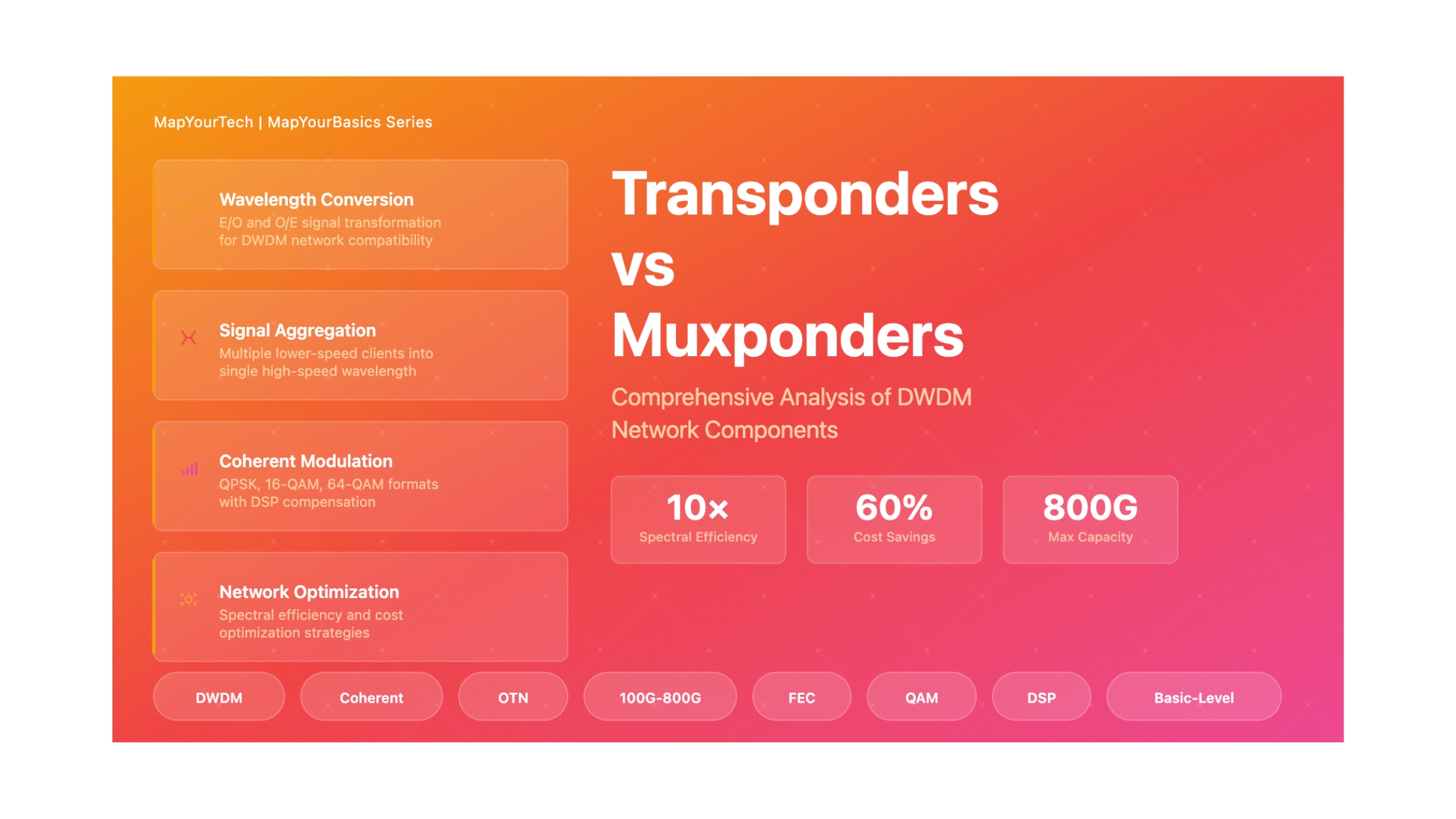
Transponders vs Muxponders
A Comprehensive Technical Guide to DWDM Network Components
Fundamentals & Core Concepts
What are Transponders?
A transponder is a key component in a DWDM system responsible for converting client data signals into optical wavelengths that can be transmitted over a DWDM network. It performs both electrical-to-optical (E/O) and optical-to-electrical (O/E) conversions.
What are Muxponders?
A muxponder combines (multiplexes) multiple lower-speed client signals into a single higher-speed wavelength for transmission over the DWDM system. It performs both E/O and O/E conversions for each individual client signal while aggregating them onto a single wavelength.
Key Differences at a Glance
Transponder Function
Protocol conversion and wavelength translation: Takes a single client signal and converts it to a WDM wavelength without aggregation.
Example: Converting a 100G Ethernet signal to an optical wavelength for DWDM transmission.
Muxponder Function
Aggregation and multiplexing: Combines multiple lower-speed signals into a single higher-speed optical wavelength.
Example: Aggregating 10× 10G Ethernet signals into a single 100G wavelength.
Why Does This Matter?
Network Efficiency: The choice between transponders and muxponders directly impacts spectral efficiency, capacity utilization, and overall network cost. Transponders provide flexibility for single high-speed services, while muxponders maximize fiber utilization by aggregating multiple lower-speed services.
Real-World Analogy: Think of a transponder as a direct flight from one city to another, while a muxponder is like a bus that picks up passengers from multiple stops before traveling to the destination—both get you there, but the muxponder consolidates multiple sources.
When Does It Matter?
- Network Planning: Choosing the right device affects capacity, cost, and scalability
- Service Type: Single high-speed vs. multiple lower-speed services
- Cost Optimization: Muxponders reduce wavelength count and associated costs
- Latency Requirements: Transponders have lower latency than muxponders
- Future Scalability: Different expansion paths and flexibility
Mathematical Framework
Line Rate Capacity:
C = R × M × N_pol × (1 - FEC_OH)
Where:
- C = Total capacity (bps)
- R = Symbol rate (GBaud)
- M = Modulation order (bits/symbol): QPSK=2, 16-QAM=4, 64-QAM=6
- N_pol = Number of polarizations (typically 2)
- FEC_OH = Forward Error Correction overhead (typically 0.07 to 0.20)
Example Calculation:
For a 400G coherent transponder using 16-QAM:
R = 64 GBaud
M = 4 bits/symbol (16-QAM)
N_pol = 2
FEC_OH = 0.15 (15% overhead)
C = 64 × 4 × 2 × (1 - 0.15)
C = 64 × 4 × 2 × 0.85
C = 435.2 Gbps gross (400G net)
Total Aggregated Capacity:
C_total = Σ(C_i) where i = 1 to N
Where:
- C_total = Total aggregated capacity
- C_i = Capacity of individual client signal i
- N = Number of client signals
Example Calculation:
10G to 100G Muxponder:
N = 10 clients
C_i = 10 Gbps each
C_total = 10 × 10 Gbps = 100 Gbps
With OTN overhead:
Line Rate = C_total / (1 - OH_otn)
Line Rate = 100 / (1 - 0.07) = 107.5 Gbps
Spectral Efficiency (SE):
SE = C / BW
Where:
- SE = Spectral efficiency (bits/s/Hz)
- C = Channel capacity (bps)
- BW = Optical bandwidth (Hz)
Comparison:
Transponder (100G, 50 GHz spacing):
SE = 100 Gbps / 50 GHz = 2 bits/s/Hz
Muxponder (10×10G on 100G, 50 GHz spacing):
SE = 100 Gbps / 50 GHz = 2 bits/s/Hz
(Same SE, but uses fewer wavelengths)
Link Budget:
P_rx = P_tx - L_total + G_amp
Where:
- P_rx = Received power (dBm)
- P_tx = Transmitted power (dBm)
- L_total = Total loss (fiber + connectors + components) (dB)
- G_amp = Amplifier gain (dB)
Example:
P_tx = 0 dBm (transponder output)
L_fiber = 0.25 dB/km × 80 km = 20 dB
L_connector = 6 dB (mux/demux)
L_margin = 3 dB (aging/repair)
G_amp = 20 dB (EDFA)
P_rx = 0 - 20 - 6 - 3 + 20 = -9 dBm
Required sensitivity: -18 dBm
System margin: -9 - (-18) = 9 dB ✓
Types & Components
Transponder Types
1. Non-Coherent Transponders
Modulation: On-Off Keying (OOK), Differential Phase Shift Keying (DPSK)
Data Rates: Up to 40 Gbps
Reach: < 120 km
Applications: Metro networks, short-reach interconnects
Advantages:
- Lower cost
- Lower power consumption (5-15W)
- Simpler design
- Lower latency
Disadvantages:
- Limited reach
- Lower spectral efficiency (0.5-1 bit/s/Hz)
- Limited dispersion tolerance
2. Coherent Transponders
Modulation: QPSK, 8-QAM, 16-QAM, 64-QAM
Data Rates: 100G, 200G, 400G, 800G+
Reach: > 1000 km (QPSK), 600+ km (16-QAM)
Applications: Long-haul, submarine, high-capacity DCI
Key Features:
- Digital Signal Processing (DSP)
- Chromatic dispersion compensation
- Polarization mode dispersion (PMD) compensation
- Soft-decision FEC (11-13 dB coding gain)
- Flexible modulation formats
Advantages:
- Extended reach (up to 4000 km)
- High spectral efficiency (2-6 bits/s/Hz)
- Superior impairment tolerance
- Adaptive modulation
Disadvantages:
- Higher cost
- Higher power consumption (10-30W)
- Complex design
- Higher OSNR requirements
3. Tunable Transponders
Wavelength Range: Full C-band (1530-1565 nm), L-band (1565-1625 nm)
Tuning Range: 40-96 channels (50 GHz spacing)
Features:
- Dynamic wavelength allocation
- Reduced spare inventory
- Network flexibility
- Software-defined wavelength provisioning
Wavelength Stability: ±0.01 nm (±1.25 GHz at 1550 nm)
Muxponder Types
| Type | Client Signals | Line Rate | Applications | Key Benefits |
|---|---|---|---|---|
| 10G to 100G | 10× 10GE | 100G | Metro, enterprise | Cost-efficient aggregation |
| 25G to 100G | 4× 25GE | 100G | Data centers | High-speed aggregation |
| 100G to 400G | 4× 100GE | 400G | Long-haul, DCI | Maximum capacity |
| Elastic Muxponder | Variable rates | Adaptive | Flexible optical networks | Energy efficiency, traffic adaptation |
Component Comparison
| Parameter | Transponder | Muxponder |
|---|---|---|
| Primary Function | Wavelength conversion | Aggregation + wavelength conversion |
| Client Ports | Single high-speed | Multiple lower-speed |
| Protocol Support | Protocol agnostic | Multi-protocol |
| Latency | Lower (μs) | Higher (due to aggregation) |
| Wavelength Usage | 1:1 (one wavelength per service) | N:1 (multiple services per wavelength) |
| Spectral Efficiency | Service-dependent | Higher (consolidation) |
| Flexibility | High (modulation, reach) | Moderate (fixed aggregation ratios) |
| Cost per Wavelength | Higher | Lower (shared resources) |
| Management | Simple | More complex |
Effects & Impacts
Network-Level Impact Analysis
Transponder Impact
Capacity: Maximum single-wavelength capacity
Flexibility: Independent service provisioning
Wavelength Consumption: Higher (1:1 ratio)
Cost Structure: Higher per wavelength, lower complexity
Performance: Optimal for high-speed services
Muxponder Impact
Capacity: Efficient aggregation of lower speeds
Flexibility: Grouped service management
Wavelength Consumption: Lower (N:1 ratio)
Cost Structure: Lower per wavelength, higher complexity
Performance: Optimal for multiple lower-speed services
Performance Impact Factors
1. Latency Impact
Transponder: Typical latency: 5-20 μs
- E/O conversion: ~2 μs
- FEC encoding/decoding: 3-10 μs
- Minimal processing overhead
Muxponder: Typical latency: 20-100 μs
- Client aggregation: 10-50 μs
- OTN framing: 5-20 μs
- Multiplexing overhead: 5-30 μs
Impact Level: Moderate - Critical for low-latency applications
2. Spectral Efficiency Impact
Scenario: Transmitting 100 Gbps total capacity
Option A: 10× 10G Transponders
- Wavelengths required: 10
- Spectrum used: 10 × 50 GHz = 500 GHz
- Overall SE: 100 Gbps / 500 GHz = 0.2 bits/s/Hz
Option B: 1× 100G Muxponder (10×10G clients)
- Wavelengths required: 1
- Spectrum used: 50 GHz
- Overall SE: 100 Gbps / 50 GHz = 2 bits/s/Hz
Efficiency Gain: 10× improvement with muxponder
3. Cost Impact Analysis
| Cost Component | 10× 10G Transponders | 1× 100G Muxponder |
|---|---|---|
| Equipment (CAPEX) | Higher (10 devices) | Lower (1 device) |
| Wavelength allocation | 10 wavelengths | 1 wavelength |
| Amplification | Higher power budget | Lower power budget |
| Management (OPEX) | 10× management points | 1× management point |
| Power consumption | 10× individual consumption | Consolidated consumption |
Typical Cost Savings: 40-60% with muxponder approach
4. Reach Impact
Coherent Transponder:
- QPSK modulation: 1000-4000 km
- 16-QAM modulation: 600-1000 km
- 64-QAM modulation: 300-600 km
Muxponder:
- Uses same transponder technology
- Reach determined by line-side optics
- No reach penalty from aggregation
- Can leverage coherent technology for extended reach
System Tolerance Thresholds
| Parameter | Non-Coherent | Coherent | Impact |
|---|---|---|---|
| Chromatic Dispersion | ±800 ps/nm | ±100,000 ps/nm | Critical |
| PMD Tolerance | 10-20 ps | 50-100 ps | High |
| OSNR Requirement | 12-15 dB | 15-25 dB (format-dependent) | Moderate |
| Wavelength Stability | ±0.05 nm | ±0.01 nm | Important |
Techniques & Solutions
Implementation Methods
1. Transponder Implementation Techniques
A. Tunable Laser Technology
- External Cavity Laser (ECL): Wide tuning range (40+ nm), precise wavelength control
- Distributed Feedback (DFB): Fixed wavelength, high stability, lower cost
- Micro-Electro-Mechanical Systems (MEMS): Fast tuning, compact design
Best Practice: Use tunable lasers for operational flexibility and reduced sparing requirements
B. Modulation Techniques
- Direct Modulation: Simple, low-cost, limited to lower speeds
- External Modulation: Mach-Zehnder modulators, higher speeds, better performance
- Coherent Modulation: IQ modulators, highest performance, complex
C. Forward Error Correction (FEC)
- Hard-Decision FEC: Reed-Solomon, 6-7 dB coding gain
- Soft-Decision FEC: LDPC, Turbo codes, 11-13 dB coding gain
- Overhead Range: 7% (standard) to 20% (enhanced)
2. Muxponder Implementation Techniques
A. Client Aggregation Methods
- Time-Division Multiplexing (TDM): OTN ODU multiplexing hierarchy
- Statistical Multiplexing: Efficient bandwidth utilization
- Flexible ODU: ODUflex for variable-rate containers
B. OTN Framing Structure
- OPU (Optical Payload Unit): Carries client data
- ODU (Optical Data Unit): Switching and routing layer
- OTU (Optical Transport Unit): FEC and line-side transmission
C. Elastic Aggregation
- Variable Bit Rate per Lane: Adapts to traffic fluctuations
- Lane Switching: Turn off unused lanes for energy savings
- Energy Proportional: Power consumption scales with traffic
Comparison of Approaches
| Technique | Advantages | Disadvantages | Best Use Case |
|---|---|---|---|
| Fixed Wavelength Transponder |
• Lowest cost • High stability • Simple deployment |
• Large spare inventory • Limited flexibility • Manual provisioning |
Static networks with no wavelength changes |
| Tunable Transponder |
• Reduced sparing • Network flexibility • Software provisioning |
• Higher cost • Wavelength stability challenges • Temperature sensitivity |
Dynamic networks, automated provisioning |
| Fixed Muxponder |
• Efficient aggregation • Lower wavelength count • Simplified management |
• Fixed aggregation ratios • Limited scalability • Single point of failure |
Stable multi-service aggregation |
| Elastic Muxponder |
• Energy efficient • Traffic adaptive • Variable bit rate |
• Higher complexity • Higher cost • Advanced control required |
Variable traffic, energy-sensitive deployments |
Best Practices and Recommendations
For Transponder Deployment
- Use tunable lasers to reduce operational complexity and sparing costs
- Select modulation format based on reach requirements (QPSK for long-haul, 16-QAM for regional)
- Implement strong FEC (15-20% overhead) for extended reach
- Monitor wavelength stability within ±0.01 nm to prevent crosstalk
- Plan for sufficient OSNR based on modulation format requirements
- Deploy protection schemes (1+1 or 1:1) for critical services
For Muxponder Deployment
- Group similar services to simplify management and provisioning
- Plan aggregation ratios considering future service additions
- Implement OTN grooming for efficient bandwidth utilization
- Use hierarchical ODU multiplexing (ODU0→ODU1→ODU2→ODU4)
- Monitor per-client performance to isolate service issues
- Consider latency requirements when selecting aggregation depth
Real-World Application Scenarios
Scenario 1: Long-Haul Network (> 1000 km)
Solution: Coherent transponders with QPSK modulation
Configuration:
- 400G coherent transponder
- QPSK or 8-QAM modulation
- 20% FEC overhead
- Tunable C-band lasers
- EDFA amplification every 80-100 km
Performance: Reach up to 2000 km without regeneration, spectral efficiency 2-3 bits/s/Hz
Scenario 2: Metro Network with Multiple Enterprises
Solution: 10G to 100G muxponder
Configuration:
- 10× 10GE client interfaces
- 1× 100G DWDM line interface
- OTN multiplexing (10× ODU2 into ODU4)
- 7% FEC overhead
- Reach: 200-400 km
Benefits: 90% reduction in wavelength count, simplified fiber management, lower cost per service
Scenario 3: Data Center Interconnect (DCI)
Solution: 100G to 400G coherent transponder or muxponder
Configuration Options:
Option A (Transponder):
- 1× 400GE client
- 1× 400G DWDM line (16-QAM)
- Maximum capacity, low latency
Option B (Muxponder):
- 4× 100GE clients
- 1× 400G DWDM line
- Service aggregation, flexible provisioning
Selection Criteria: Choose transponder for single 400G service, muxponder for multiple 100G services
Design Guidelines & Methodology
Decision Framework: Transponder vs Muxponder
Step-by-Step Selection Process
Step 1: Analyze Service Requirements
- Number of services to transport
- Individual service rates (10G, 100G, 400G)
- Total aggregate capacity needed
- Service growth projections (3-5 years)
- Latency requirements
Step 2: Evaluate Network Characteristics
- Distance between sites
- Fiber type and condition
- Available spectrum
- Existing infrastructure
- OSNR budget
Step 3: Calculate Cost-Benefit
- CAPEX: Equipment costs
- OPEX: Power, cooling, management
- Wavelength licensing costs
- Sparing requirements
- Total cost of ownership (TCO)
Step 4: Apply Decision Rules
Choose Transponder When:
- ✓ Single high-speed service (100G, 400G, 800G)
- ✓ Ultra-low latency required (< 20 μs)
- ✓ Maximum flexibility needed
- ✓ Independent service lifecycle management
- ✓ Long-reach requirements (> 1000 km)
- ✓ Maximum per-wavelength capacity needed
- ✓ Service rate matches line rate (e.g., 100G client → 100G line)
Choose Muxponder When:
- ✓ Multiple lower-speed services (10G, 25G, 100G)
- ✓ Spectral efficiency is priority
- ✓ Minimizing wavelength count is critical
- ✓ Services have common source/destination
- ✓ Latency tolerance > 50 μs
- ✓ Cost optimization through aggregation
- ✓ Simplified network management preferred
Design Methodology
Requirements:
- 15× 10GE services between two cities
- Distance: 350 km
- Latency requirement: < 100 μs
- 5-year growth: +50% capacity
Option 1: Individual 10G Transponders
Equipment: 15× 10G transponders
Wavelengths: 15
Spectrum: 15 × 50 GHz = 750 GHz
Amplifiers: 4 sites × 15 wavelengths = 60 amplifier channels
Power budget: 15 × 20W = 300W
Estimated CAPEX: $375,000 (15 × $25,000)
Annual OPEX: $45,000
Option 2: 100G Muxponder (10×10G aggregation)
Equipment: 2× 100G muxponders (10×10G each)
Wavelengths: 2
Spectrum: 2 × 50 GHz = 100 GHz
Amplifiers: 4 sites × 2 wavelengths = 8 amplifier channels
Power budget: 2 × 40W = 80W
Estimated CAPEX: $140,000 (2 × $70,000)
Annual OPEX: $12,000
Savings: 62% CAPEX, 73% OPEX, 87% spectrum
Recommendation: Choose Muxponder Option
Justification: Significant cost and spectrum savings, latency acceptable, services have common endpoints
Design Checklist
Transponder Design Checklist
- ☑ Link budget calculated and verified
- ☑ Modulation format selected based on reach
- ☑ FEC overhead planned (7-20%)
- ☑ OSNR requirements met (15-25 dB)
- ☑ Dispersion compensation validated
- ☑ Wavelength plan assigned
- ☑ Protection scheme defined (if required)
- ☑ Power budget with margin (3-5 dB)
- ☑ Temperature operating range verified
- ☑ Management interfaces configured
Muxponder Design Checklist
- ☑ Client services identified and grouped
- ☑ Aggregation ratio verified (e.g., 10×10G→100G)
- ☑ OTN hierarchy planned (ODU mapping)
- ☑ Total latency budget calculated
- ☑ Client interface types confirmed
- ☑ Line-side optics selected
- ☑ Grooming strategy defined
- ☑ Failover behavior specified
- ☑ Per-client monitoring enabled
- ☑ Growth capacity planned (20% minimum)
Common Pitfalls to Avoid
Transponder Deployment Mistakes
- ❌ Insufficient OSNR margin: Always add 3-5 dB margin for aging and repairs
- ❌ Wrong modulation selection: Don't use 64-QAM for long-reach applications
- ❌ Ignoring dispersion: Coherent transponders compensate CD, but verify PMD tolerance
- ❌ Fixed wavelength over-reliance: Use tunable for flexibility unless cost prohibitive
- ❌ Inadequate FEC: Balance overhead vs. coding gain for your application
- ❌ No protection planning: Define 1+1 or 1:1 schemes for critical services
Muxponder Deployment Mistakes
- ❌ Over-aggregation: Don't fill all ports at deployment—leave 20% growth capacity
- ❌ Mixing incompatible services: Group services with similar QoS requirements
- ❌ Ignoring latency: Aggregation adds 30-80 μs—verify application tolerance
- ❌ Single point of failure: One muxponder failure affects all aggregated services
- ❌ Poor grooming strategy: Plan ODU hierarchy carefully to avoid stranded capacity
- ❌ Inadequate per-client monitoring: Ensure individual service performance visibility
🎮 Interactive Simulators
Practical Applications & Case Studies
Case Study 1: Global Financial Services Network
Challenge
A multinational bank needed to interconnect 50 branches with low-latency connectivity for trading applications. Each branch required 10 Gbps connectivity, with ultra-low latency requirements (< 30 μs per hop) for high-frequency trading.
Solution Approach
Selected: Individual 10G Coherent Transponders
Rationale:
- Latency requirement eliminated muxponder option (would add 50-80 μs)
- Each branch needed independent wavelength management
- Service-level SLA required per-branch monitoring
- Long distances (300-800 km) required coherent technology
Implementation Details
- Equipment: 50× 10G coherent transponders with QPSK modulation
- Reach: Up to 1200 km without regeneration
- Latency: 12 μs per transponder (within requirements)
- Protection: 1+1 optical protection for all links
- Management: SDN controller for automated wavelength provisioning
Results & Benefits
- ✓ Achieved < 25 μs latency per hop
- ✓ 99.999% availability with protection switching
- ✓ Independent service management per branch
- ✓ Flexible bandwidth upgrades without affecting other branches
- ✓ ROI achieved in 2.5 years through trading efficiency gains
Case Study 2: Regional ISP Metro Aggregation
Challenge
A regional ISP needed to aggregate traffic from 120 enterprise customers (each with 10 GE) across 12 metro aggregation points to 3 core data centers. Cost optimization was critical, with limited spectrum availability.
Solution Approach
Selected: 100G Muxponders (10×10G aggregation)
Rationale:
- Spectral efficiency: 92% reduction in wavelength count
- Cost optimization: 65% CAPEX savings vs. individual transponders
- Latency acceptable for enterprise services (< 100 μs)
- Simplified management with consolidated wavelengths
Implementation Details
- Equipment: 12× 100G muxponders at metro sites
- Aggregation: 10× 10GE clients per muxponder
- Line rate: 100G with 7% FEC overhead
- Distance: 150-300 km to core
- Technology: OTN multiplexing (ODU2→ODU4)
Results & Benefits
- ✓ Reduced from 120 wavelengths to 12 wavelengths (90% reduction)
- ✓ $4.2M CAPEX savings over 3 years
- ✓ 78% reduction in power consumption
- ✓ Simplified fiber management across metro network
- ✓ Easy service provisioning using OTN grooming
- ✓ 20% spare capacity for growth
Case Study 3: Submarine Cable System
Challenge
A submarine cable consortium needed to build a 4,500 km transoceanic link with maximum capacity (16 Tbps) and minimal cost per bit. Ultra-long reach without regeneration was essential to reduce underwater equipment.
Solution Approach
Selected: 400G Coherent Transponders with QPSK modulation
Rationale:
- Maximum reach requirement (> 4000 km) mandated coherent QPSK
- High capacity per wavelength to maximize fiber utilization
- Soft-decision FEC with 12 dB coding gain for extended reach
- No muxponder option—line-side already at maximum capacity
Implementation Details
- Equipment: 40× 400G coherent transponders per fiber pair
- Modulation: DP-QPSK for maximum reach
- FEC: 20% overhead soft-decision FEC
- Symbol rate: 64 GBaud
- Capacity: 400G gross, 333G net per wavelength
- Total capacity: 16 Tbps per fiber pair (40 wavelengths)
- Amplification: EDFA every 50-80 km
Results & Benefits
- ✓ Achieved 4,500 km reach without regeneration
- ✓ 16 Tbps total capacity across 40 wavelengths
- ✓ 40% cost reduction vs. previous generation (100G)
- ✓ Spectral efficiency: 3.2 bits/s/Hz
- ✓ 25-year design life with upgrade path to 800G
- ✓ BER maintained at < 10^-15 across entire link
Troubleshooting Guide
| Problem | Possible Causes | Diagnosis | Solution |
|---|---|---|---|
| High BER on Transponder |
• Insufficient OSNR • Excessive dispersion • Fiber nonlinearity • Wavelength drift |
• Measure OSNR • Check dispersion • Verify power levels • Monitor wavelength |
• Adjust amplifier gain • Enable DSP compensation • Reduce launch power • Stabilize wavelength |
| Muxponder Client Loss |
• Client interface failure • OTN mapping error • Clock synchronization • Card failure |
• Check client port LEDs • Verify ODU mapping • Check alarms (LOS, LOF) • Test loopback |
• Replace client optics • Reconfigure OTN mapping • Synchronize clocks • Replace line card |
| Wavelength Drift |
• Temperature variation • Laser aging • Insufficient control • TEC failure |
• Monitor wavelength • Check temperature • Verify TEC operation • Check wavelength locker |
• Improve cooling • Calibrate laser • Enable wavelength locker • Replace TEC |
| Excessive Latency (Muxponder) |
• Deep aggregation • FEC overhead • Processing delay • Buffering |
• Measure end-to-end latency • Check aggregation depth • Verify FEC settings • Monitor queue depths |
• Reduce aggregation ratio • Lower FEC overhead • Optimize DSP • Clear buffers |
| Crosstalk Between Channels |
• Insufficient channel spacing • Filter misalignment • Excessive power • Nonlinear effects |
• Measure channel isolation • Check filter response • Monitor power spectrum • Verify channel plan |
• Increase channel spacing • Align filters • Reduce power levels • Respace channels |
Quick Reference: Decision Matrix
| Scenario | Recommended Solution | Key Consideration |
|---|---|---|
| Single 100G/400G service | Transponder | Simplicity, low latency |
| Multiple 10G services, same route | Muxponder | Cost efficiency, spectrum savings |
| Ultra-low latency (< 20 μs) | Transponder | Minimal processing delay |
| Long-haul (> 1000 km) | Coherent Transponder | Extended reach capability |
| Metro aggregation (< 500 km) | Muxponder | Cost optimization |
| Spectrum constrained | Muxponder | Wavelength consolidation |
| Independent service management | Transponder | Per-service flexibility |
| Maximum fiber utilization | Muxponder | Aggregation efficiency |
Professional Recommendations
For Network Planners
- Start with requirements: Clearly define capacity, latency, reach, and cost targets
- Plan for growth: Allocate 20-30% spare capacity
- Consider TCO: Include CAPEX, OPEX, power, and management costs
- Evaluate hybrid approaches: Mix transponders and muxponders as needed
- Use tunable technology: Maximize operational flexibility
- Implement monitoring: Comprehensive performance visibility
For Network Operators
- Document wavelength plans: Maintain accurate records
- Monitor proactively: Track OSNR, BER, and power levels
- Maintain spares: Keep critical components in inventory
- Train staff: Ensure team understands both technologies
- Update procedures: Document troubleshooting workflows
- Plan maintenance windows: Schedule regular testing

Optical Communications & Network Automation Expert | Author of 3 Books for Optical Engineers | Founder, MapYourTech
Optical networking engineer with nearly two decades of experience across DWDM, OTN, coherent optics, submarine systems, and cloud infrastructure. Founder of MapYourTech. Read full bio →
Follow on LinkedInRelated Articles on MapYourTech