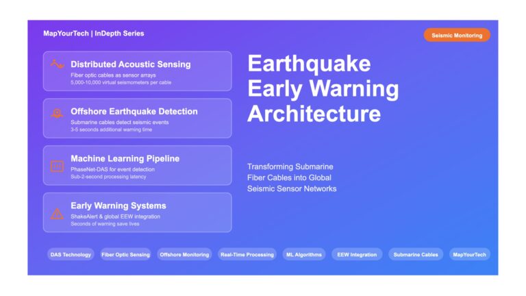
Earthquake Early Warning System Architecture: A Visual Technical Guide | MapYourTech Earthquake Early Warning System Architecture Transforming Submarine Fiber Optic...
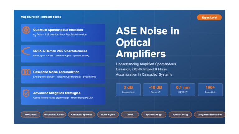
ASE Noise in Optical Amplifiers: Understanding Amplified Spontaneous Emission, OSNR Impact, and Cascaded Amplifier Noise Accumulation – Expert Deep Dive...
Reliability Engineering for Subsea Cable Systems Reliability Engineering for Subsea Cable Systems Submarine Communications | Network Engineering Introduction Subsea cable...
In-House vs Merchant DSP Architectures in Coherent Optical Networks | MapYourTech In-House vs Merchant DSP Architectures in Coherent Optical Networks...