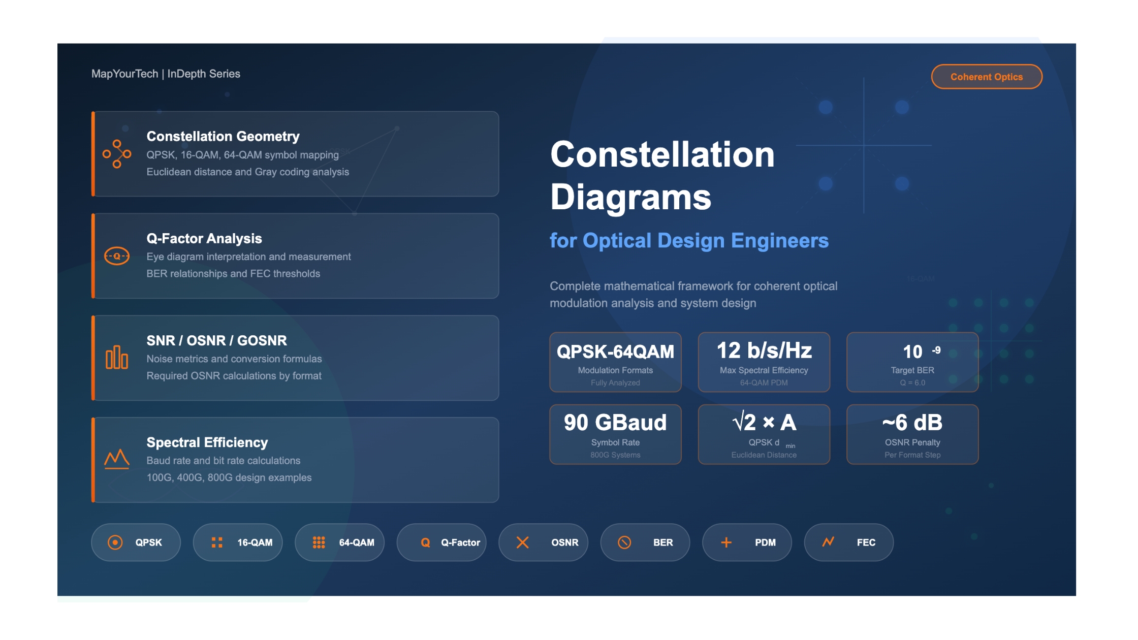
Complete Guide to Constellation Diagrams for Optical Design Engineers

Understanding QPSK and QAM: Euclidean Distance, SNR, OSNR, Q-Factor, and System Design Calculations

1. Introduction to Constellation Diagrams

A constellation diagram is a two-dimensional representation of a digital modulation scheme in the complex signal space, where the horizontal axis represents the In-phase (I) component and the vertical axis represents the Quadrature (Q) component. Each point in the constellation corresponds to a unique symbol that carries one or more bits of information. The position of each symbol is defined by its amplitude and phase relative to the carrier signal.

In coherent optical communication systems, the electric field of the optical signal can be expressed as:

Es(t) = As(t) × exp(jωst)

Where:
  As(t)  = Complex signal amplitude (I + jQ components)
  ωs     = Angular frequency of the modulated optical signal
  t      = Time

The complex amplitude A_s(t) = I(t) + jQ(t) determines the position of the signal in the constellation diagram. Coherent detection using a local oscillator allows recovery of both amplitude and phase information, enabling the use of advanced modulation formats such as QPSK, 16-QAM, and 64-QAM.

2. QPSK Constellation: Complete Analysis

2.1 QPSK Symbol Definition

Quadrature Phase-Shift Keying (QPSK) is a four-state modulation format where data is encoded onto two orthogonal components of the signal. Each symbol represents 2 bits of information. In coherent optical systems, QPSK combined with polarization-division multiplexing (PDM-QPSK) is widely used for 100G transmission systems.

2.2 QPSK Mathematical Definition

For QPSK modulation, the four symbols are positioned at equal angles of 45°, 135°, 225°, and 315° from the positive I-axis. The modulated signal can be expressed as:

x(t) = A × cos(2πf0t + φk)

Phase values for QPSK (k = 0, 1, 2, 3):
  φk = (2k + 1) × π/4
  
  φ0 = 45°  (π/4)    → Symbol "00"
  φ1 = 135° (3π/4)   → Symbol "01"  
  φ2 = 225° (5π/4)   → Symbol "11"
  φ3 = 315° (7π/4)   → Symbol "10"

Symbol coordinates (I, Q):
  S0 = (A/√2, A/√2)
  S1 = (-A/√2, A/√2)
  S2 = (-A/√2, -A/√2)
  S3 = (A/√2, -A/√2)