
 MapYourTech | InDepth Series
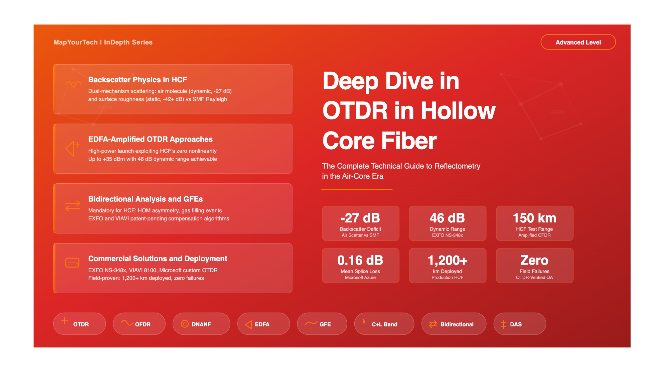
Deep Dive in OTDR in Hollow Core Fiber: The Complete Technical Guide to Reflectometry in the Air-Core Era
How the 30 dB backscatter deficit is reshaping every assumption about optical time domain reflectometry -- and the engineering innovations closing the gap for production HCF networks.
1.0 Introduction -- OTDR Meets the Hollow Revolution
Optical Time Domain Reflectometry (OTDR) has been the foundation of fiber optic network characterization and maintenance for over four decades. Every fiber installation, every splice verification, and every fault-finding exercise in the global optical network relies on the same basic principle: send a short pulse of light into a fiber, measure the tiny fraction that scatters back, and reconstruct a map of events and losses along the link. In standard single-mode fiber (SMF), this process is well understood, highly optimized, and supported by mature commercial instruments and international standards.
Hollow Core Fiber (HCF) changes nearly every assumption that makes conventional OTDR work. Because light in HCF travels through an air-filled core rather than through solid silica glass, the Rayleigh backscattering mechanism that generates the OTDR trace in standard fiber is reduced by approximately 27 to 30 dB. This is not a minor calibration adjustment. It represents a reduction of roughly three to four orders of magnitude in the returned signal power that an OTDR instrument must detect and process. In practical terms, it means that a conventional field OTDR, configured for standard SMF, produces an unusable trace when connected to a hollow core fiber -- the backscatter level falls below the instrument's noise floor within a few hundred meters, and events such as splices become invisible.
The timing of this challenge could not be more critical. As of early 2026, hollow core fiber has moved decisively from the research laboratory into production networks. Microsoft has deployed over 1,200 km of DNANF (Double Nested Anti-Resonant Nodeless Fiber) carrying live Azure customer traffic and announced plans to install 15,000 km across its global cloud infrastructure. AWS, Chinese operators including China Mobile, and financial trading firms are following with their own deployments. These networks require the same rigorous testing and certification workflows that operators apply to SMF infrastructure: verifying splice quality, locating faults, measuring attenuation, and performing ongoing maintenance. Without reliable reflectometry, operators cannot validate their HCF installations or troubleshoot problems in the field.
The central challenge of OTDR in HCF is not that backscatter is absent -- it is that the scattering originates from fundamentally different physical mechanisms than in solid-core fiber, each with distinct characteristics that affect OTDR trace interpretation. Understanding these mechanisms is essential for any engineer working with HCF deployment or testing.
This article provides a comprehensive technical examination of OTDR technology as it applies to hollow core fiber. It covers the fundamental physics of backscattering in HCF, the engineering approaches that have been developed to overcome the dynamic range deficit, the new analysis algorithms required for accurate trace interpretation, and the commercial test solutions that have emerged in 2025-2026 from vendors such as EXFO and VIAVI. It also examines complementary techniques including Optical Frequency Domain Reflectometry (OFDR) and the specialized OTDR Microsoft developed for its own Azure HCF deployments. The objective is to equip optical network engineers, system designers, and researchers with the knowledge needed to effectively characterize and maintain HCF links using reflectometry.
2.0 OTDR Fundamentals: A Refresher for the HCF Context
Before examining the challenges HCF introduces, a brief review of how conventional OTDR operates in standard fiber establishes the baseline assumptions that HCF disrupts.
2.1 Operating Principle
An OTDR injects short optical pulses into one end of a fiber and measures the optical power returning to the same end as a function of time. This returned power comes from two distinct sources: Rayleigh backscattering (RBS), which is a continuous process occurring at every point along the fiber, and Fresnel reflections, which are discrete events occurring at interfaces where the refractive index changes abruptly, such as connectors, splices with air gaps, or fiber end-faces.
The time delay between the launched pulse and each returned signal directly corresponds to a position along the fiber, since light travels at a known speed determined by the fiber's refractive index. The instrument converts these time-domain measurements into a spatial trace showing optical power (in dB) versus distance. On this trace, the continuous Rayleigh backscatter appears as a gradually declining line (whose slope represents the fiber's attenuation coefficient), while Fresnel reflections appear as sharp upward spikes.
Figure 1: OTDR operating principle showing pulse launch, backscatter collection, and the resulting trace with characteristic events including connector reflections, splice losses, and fiber end reflection.
2.2 Critical OTDR Parameters
Several parameters define an OTDR's capability for a given measurement task. Dynamic range is the most critical for HCF applications -- it represents the difference between the backscatter level at the launch point and the instrument's noise floor, typically specified at a signal-to-noise ratio (SNR) of 1. Higher dynamic range enables measurements over longer distances or through higher-loss links. In standard SMF, Rayleigh backscatter at 1550 nm is approximately -72 dB/m relative to the launched power. Typical field OTDRs provide 35 to 45 dB of dynamic range, sufficient for characterizing links of 100 km or more.
Pulse width determines the trade-off between spatial resolution and dynamic range. Shorter pulses enable finer resolution (the ability to distinguish closely spaced events) but carry less energy, reducing the range. Longer pulses extend range but create larger dead zones after reflective events. Dead zones -- both event dead zones (the minimum distance between two reflective events that can be separately detected) and attenuation dead zones (the minimum distance after a reflection where the OTDR can measure attenuation accurately) -- define the instrument's ability to resolve closely spaced network elements.
The Index of Refraction (IOR) setting converts time-of-flight to distance. For standard SMF at 1550 nm, the group index is approximately 1.4677. This value differs significantly for HCF, where the core is air, and must be configured correctly to obtain accurate distance measurements.
Distance = (c x t) / (2 x ng)

Where:
  c   = speed of light in vacuum (2.998 x 10⁸ m/s)
  t   = round-trip time of flight (seconds)
  ng  = group refractive index of the fiber core

-- For SMF:  n_g ~ 1.4677 at 1550 nm
-- For HCF:  n_g ~ 1.0003 (air core, near vacuum)

-- The factor of 2 accounts for the round-trip path
-- Light travels ~47% faster in HCF than in SMFRead the Full Analysis with Premium
The remaining 89% of this article — the design numbers, trade-offs and field guidance — is part of MapYourTech Premium, along with the full premium library, courses and professional tools.



Course Title
Course description and key highlights
Course Content
Course Details
Celebrating 1,000+ LinkedIn posts
3 hours of Premium Pro, free
The full Premium Pro library, unlocked with one click. The clock starts the moment you check out and runs for 3 full hours - pick a time when you can make the most of it.
- Courses
- Interview preparation content
- Career development posts
- Simulators
- Calculators
- Market research
No card, nothing to cancel. One pass per person. Sign in or create a free account at checkout.
Follow MapYourTech on LinkedIn for regular updates and future promos.
New articles, tool releases and member offers, posted as they go live.
Follow MapYourTech on LinkedIn
Enjoying MapYourTech? Follow us on LinkedIn. One click and this stops appearing.
- New technical articles and tool releases, posted as they go live
- Course launches and member offers before they reach the site
- Standards and industry updates worth an optical engineer's time
New articles, tool releases and member offers, posted as they go live.