
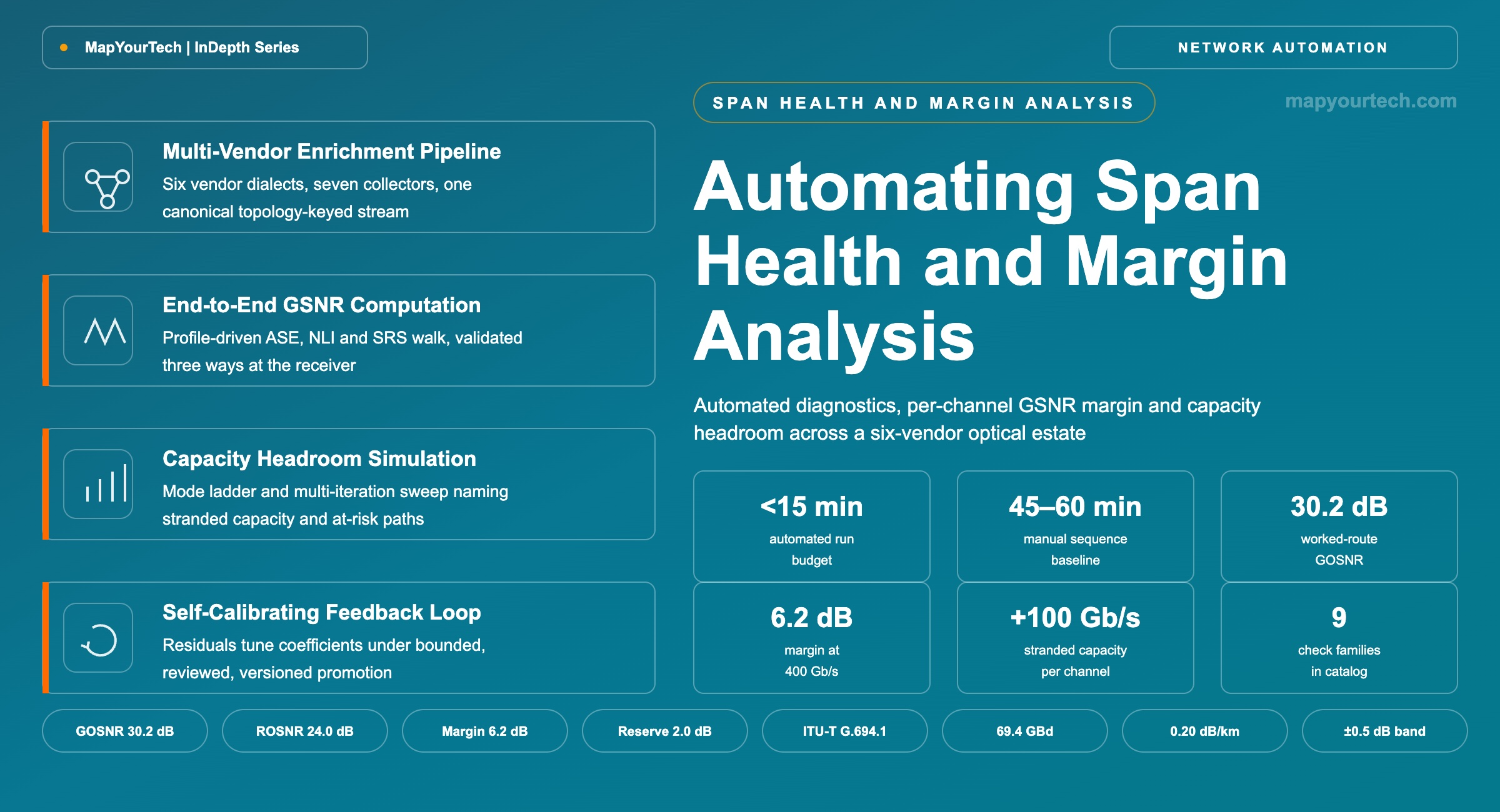
Automating Span Health and Margin Analysis in Multi-Vendor Optical Networks
A system that collects the health of every operational span across vendors and layers in under 15 minutes, computes per-channel margin from live telemetry, and reports the capacity headroom left unused in provisioned channels.
Margin you cannot name is margin you cannot spend.
What You Will Learn
- Quantify the manual diagnostic sequence a span incident triggers today — nine check families totaling a representative 45–60 minutes — against the sub-15-minute automated target of Table 1.
- Build the five-layer architecture of Figure 2 — sources, acquisition, normalization, analysis engines, presentation — with NETCONF, gNMI, SNMP and TL1 collectors feeding the six-vendor enrichment pipeline of Figure 3.
- Construct the six-level topology hierarchy of Figure 4 — service, channel, OMS, OTS, span, fiber segment — so every measurement and check attaches to exactly one level.
- Define the nine-entry health check catalog of Table 2, including the three device-level checks — protection policy state, adjacency count, neighbor identity — that no polling inventory covers.
- Compute per-channel margin from telemetry: convert a DSP-reported 22.8 dB SNR at 69.4 GBd to 30.2 dB OSNR in 0.1 nm, and subtract a 24.0 dB mode requirement for 6.2 dB of margin.
- Sweep the transceiver mode ladder of Table 7 to find hidden capacity — the worked route carries a 400G channel that closes at 500G with 1.7 dB of residual margin after a 2.0 dB planning reserve.
- Place the three trigger paths of Figure 7 — event-driven, on-demand, scheduled — around one rate-limited orchestrator so results exist before an engineer opens the incident.
- Anchor the build against the three recurring failure patterns of Section 16 — cross-connected line systems, unnoticed protection hold-down, and automation rollback conflicts — that the check catalog exists to catch.
1. Introduction
An automated span health system answers one operational question in minutes instead of an hour: what is the current state of this span, and which of its layers deserves an engineer's attention right now. This guide describes how to build such a system for inter-data-center and long-haul dense wavelength-division multiplexing (DWDM) spans in a multi-vendor network — a system that takes a region, a site pair, or a single span as input, runs every check an experienced engineer would run by hand, and returns a structured summary in under 15 minutes. The same collection machinery then feeds a second, higher-value function: per-channel margin analysis, which estimates how much quality-of-transmission headroom each provisioned channel carries in service, and reports where a channel configured at 400 Gb/s could close at 500 Gb/s or 600 Gb/s on the same fiber.
The operational problem is concrete. When a span fails, degrades, or shows triangulated packet loss, the engineer who picks up the incident faces a diagnostic sequence spread across eight to ten separate tools: the incident queue, the optical alarm view, the inventory system, the packet-loss history, the traffic and interface-error dashboards, the maintenance calendar, the deployment system, and the event logs — followed by device-level checks that no portal covers at all, run one device at a time over dozens of terminal devices. Operational experience at large operators puts that sequence at 45–60 minutes in a representative incident (a measured range from incident reviews, developed in Section 3), and the whole hour runs while customer impact is ongoing. The diagnostic time is pure discovery: nothing is fixed during it, and the checks themselves are mechanical. That combination — long, repetitive, fully specifiable — is the definition of a task that belongs in software.
The second problem is quieter and costs capacity rather than time. Coherent channels are provisioned once, at a planning margin chosen for end-of-life conditions, and then run for years without anyone re-reading their actual performance. A channel planned conservatively at 400 Gb/s on a route whose measured generalized signal-to-noise ratio (GSNR) sits 6 dB above the mode's threshold is carrying stranded capacity: a higher-rate transceiver mode would close on the same path with margin to spare. Because the health system already collects per-channel telemetry — pre-forward-error-correction (pre-FEC) bit error rate (BER), Q-factor, received power, chromatic dispersion (CD), polarization mode dispersion (PMD) — extending it into a margin and headroom engine is an increment, not a second project. The combined system is the subject of this guide.
The guide is written for the engineer who has to implement this, not evaluate it. Section 3 fixes the quantities the whole system computes; Sections 3 through 8 build the collection side: requirements, architecture, acquisition protocols, the multi-vendor enrichment pipeline, the topology model, and the health check catalog. Sections 9 through 11 build the analysis side: the monitoring-point inventory and vendor profiles, GSNR estimation and margin computation, and the multi-iteration mode simulation that surfaces hidden capacity. Sections 12 through 15 cover orchestration, report design, the self-calibrating feedback loop, and a phased implementation plan, and Section 16 closes with three recurring failure patterns from field operations that justify specific checks in the catalog. Background on the control-plane machinery used throughout is available in the optical network automation guide and the NETCONF and YANG primer on this site.
Takeaway: A span health system automates a 45–60 minute manual diagnostic sequence into a sub-15-minute structured collection run, and the same telemetry pipeline extends into per-channel margin and capacity headroom analysis at marginal additional cost.
2. Optical Margin Definition and Component Quantities
Optical margin is the headroom, in decibels, between the signal quality a channel delivers and the minimum its receiver requires: the generalized optical signal-to-noise ratio (GOSNR) achieved end to end on the path, minus the required OSNR of the provisioned mode, with both terms expressed in the same 0.1 nm reference bandwidth.
The full anatomy sits on a decibel axis in Figure 1, drawn to scale: 6.2 dB of margin between the 30.2 dB measured GOSNR and the 24.0 dB requirement, split into a 2.0 dB planning reserve and 4.2 dB of spendable headroom.
Three neighboring quantities get conflated with margin, and one sentence separates each pair. OSNR counts amplified spontaneous emission (ASE) alone, while GOSNR folds ASE and nonlinear interference (NLI) into a single ratio, which is why GOSNR rather than OSNR predicts receiver behavior. The receiver's digital signal processor (DSP) reports SNR in its own symbol-rate bandwidth, while GOSNR uses the 0.1 nm (12.5 GHz) reference, so the two describe the same channel through different windows. And margin is measured headroom above the mode's requirement, while the planning reserve is the slice of that margin allocated in advance for aging, repair splices, and fast transients — the reserve is spent by policy, the remainder by physics.
One line converts between the two bandwidth conventions: OSNR0.1nm = SNR + 10·log10(Rs / 12.5 GHz), with SNR the DSP-reported ratio in the symbol-rate bandwidth and Rs the symbol rate in GBd. At 69.4 GBd the conversion term is 10·log10(69.4/12.5) = 7.44 dB, so a DSP-reported SNR of 22.8 dB corresponds to a GOSNR-equivalent OSNR of 22.8 + 7.44 = 30.2 dB; against the 24.0 dB required OSNR of the 400 Gb/s mode that is a margin of 6.2 dB, and after the 2.0 dB planning reserve, 4.2 dB remains spendable — the reference case every later section returns to.
Takeaway: Margin is GOSNR minus required OSNR in one shared 0.1 nm reference; OSNR alone omits NLI, DSP-reported SNR sits in a different bandwidth, and the planning reserve is an allocation inside margin rather than an addition to the requirement — every later computation rests on keeping those four quantities apart.
3. Manual Diagnosis Cost and System Requirements
The manual diagnostic sequence for a span incident spans nine check families, and its representative total of 45–60 minutes is dominated by device-level verification that has no portal at all. The sequence as engineers run it today is in Table 1, with representative per-check durations drawn from incident reviews at large-scale operators (operational experience, not a standard-specified figure — individual events vary with region size and tool responsiveness). The first eight families are portal work: each is quick in isolation, but they live in eight different systems with eight different query models, and the engineer serializes them because the output of one shapes the next.
| Check Family | Source System | Representative Duration (min) |
|---|---|---|
| Incident queue review | Ticketing system | 2 |
| Optical alarm and site-record review | Optical NMS, site inventory | 5 |
| Out-of-service device check | Inventory system | 2 |
| Packet-loss history | Loss-monitoring platform | 5–10 |
| Traffic levels, interface errors, discards | Traffic telemetry dashboards | 5–15 |
| Maintenance-window review | Change calendar | 2–5 |
| Active deployment review | Deployment system | 2–5 |
| Event and log search | Log aggregation | 5 |
| Device-level state verification | Direct device sessions | 15–30 |
Read the Full Analysis with Premium
The remaining 89% of this article — the design numbers, trade-offs and field guidance — is part of MapYourTech Premium, along with the full premium library, courses and professional tools.
You May Also Like

-
Free
-
September 4, 2026

-
Premium
-
September 4, 2026

-
Premium
-
September 4, 2026