
Generic selectors
Exact matches only
Search in title
Search in content
Post Type Selectors
Articles
lp_course
lp_lesson
Back
HomeAnalysisHigh-Order Modulation Formats
High-Order Modulation Formats

High-Order Modulation Formats

Last Updated: April 2, 2026
17 min read
107
High-Order Modulation Formats, Constellation Design, and Digital Signal Processing for High-Speed Transmission Systems

High-Order Modulation Formats, Constellation Design, and Digital Signal Processing for High-Speed Transmission Systems

Executive Summary

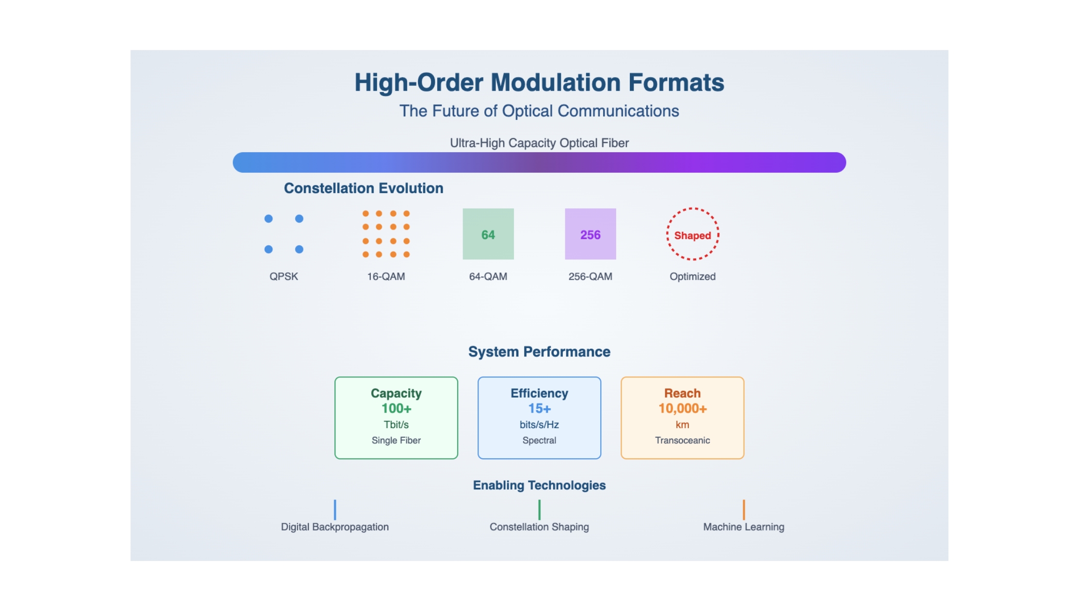
High-order modulation formats represent a critical advancement in optical fiber communication systems, enabling unprecedented data transmission rates while maximizing spectral efficiency within limited bandwidth constraints. This comprehensive analysis examines the evolution from traditional QPSK to advanced m-QAM formats (where m ≥ 64), constellation shaping techniques, and sophisticated digital signal processing algorithms that collectively address the fundamental challenge of nonlinear fiber impairments.

The convergence of probabilistic and geometrical constellation shaping with advanced forward error correction (FEC) schemes has demonstrated spectral efficiencies exceeding 7 bits/s/Hz over transoceanic distances. Key findings indicate that optimal performance requires simultaneous optimization of modulation format, code rate, and digital backpropagation bandwidth, with theoretical gains approaching the Shannon capacity limit through careful management of signal-signal and signal-noise nonlinear interactions.

Key Implications for the Field

  • Capacity Revolution: Potential for 6.25 Tbit/s additional capacity at 3200 km through full-bandwidth digital backpropagation
  • Nonlinearity Mitigation: Up to 8 dB SNR gains achievable through multichannel digital backpropagation techniques
  • Shaping Advantage: 1.53 dB theoretical gain from constellation shaping approaches Shannon capacity limits
  • Integration Complexity: EEPN (Equalization Enhanced Phase Noise) emerges as critical limiting factor in practical implementations

Historical Context & Foundational Principles

Evolution of Optical Modulation Technology

1980s - Digital Coherent Detection Foundations

Pioneering work by Ungerboeck and others established trellis-coded modulation (TCM) principles, laying groundwork for bandwidth-limited transmission regimes where unlimited power but limited bandwidth drives system design.

1990s - Fiber Nonlinearity Understanding

Recognition of the nonlinear Schrödinger equation as the fundamental model for optical fiber propagation. Key breakthrough: understanding that fiber nonlinearity follows the relationship neff = n₀ + n₂|E(t,z)|², where n₂ ≈ 3×10⁻²⁰ m²/W for silica.

2000s - Coherent Detection Renaissance

Development of digital signal processing enabling coherent optical detection with amplitude and phase recovery. Introduction of electronic dispersion compensation (EDC) and polarization mode dispersion (PMD) mitigation algorithms.

2010s - Nonlinearity Compensation Breakthrough

Digital backpropagation (DBP) emerges as viable solution for Kerr nonlinearity mitigation. Split-step Fourier method enables practical implementation of reverse propagation algorithms.

2020s - Constellation Shaping & AI Integration

Probabilistic and geometrical shaping techniques mature, achieving near-Shannon capacity performance. Machine learning begins influencing constellation design and optimization strategies.

Theoretical Frameworks Underpinning High-Order Modulation

Fundamental Nonlinear Propagation Model

The propagation of optical signals through single-mode fiber is governed by the nonlinear Schrödinger equation, which in the single polarization case is expressed as:

∂E(t,z)/∂z = -j(β₂/2)(∂²E(t,z)/∂t²) - (α/2)E(t,z) + jγ|E(t,z)|²E(t,z)

Dispersion Parameter (β₂)

Group velocity dispersion coefficient, typically -21 ps²/km for standard single-mode fiber at 1550 nm wavelength.

Attenuation (α)

Fiber loss coefficient, approximately 0.2 dB/km for modern optical fibers.

Nonlinear Coefficient (γ)

Defined as γ = k₀n₂/Aeff, typically 1.2/(W·km) where Aeff is the effective core area.

Dual-Polarization Manakov Equation

For practical fiber systems employing dual-polarization transmission, the more general Manakov equation applies:

∂E(t,z)/∂z = -j(β₂/2)(∂²E(t,z)/∂t²) - (α/2)E(t,z) + j(8/9)γ||E(t,z)||²E(t,z)

where E(t,z) represents the dual-polarization optical field vector, and the (8/9) factor accounts for the statistical averaging over polarization states in randomly birefringent fiber.

Paradigm Shifts in System Design Philosophy

Traditional Linear Compensation

  • Electronic dispersion compensation only
  • PMD equalization using CMA/LMS
  • Simple carrier phase estimation
  • Limited to ~4 bits/symbol efficiency

Modern Nonlinear Mitigation

  • Digital backpropagation with split-step FFT
  • Multichannel joint processing
  • Advanced constellation shaping
  • Achieves >12 bits/symbol efficiency

Core Physical Principles

Kerr Nonlinearity Classification

The optical Kerr effect manifests in three distinct forms, each with different implications for system design:

Self-Phase Modulation (SPM) Ch 0 φ_NL ∝ |E₀|² Intrachannel nonlinearity Cross-Phase Modulation (XPM) Ch 1 Ch 0 Ch 2 φ_NL ∝ 2(|E₁|² + |E₂|²) Interchannel nonlinearity Four-Wave Mixing (FWM) f₁ f₂ f₃ f₄ f = f₁ + f₂ - f₃ Phase matching: Δβ ≈ 0 Coherent frequency mixing

Critical Design Insight

The relative importance of SPM, XPM, and FWM depends strongly on the dispersion management strategy. In dispersion-unmanaged systems using standard single-mode fiber (SSMF), SPM and XPM dominate due to poor phase matching conditions for FWM (Δβ >> 1).

Technical Architecture & System Design

Component-Level System Architecture

Modern high-order modulation transmission systems integrate multiple sophisticated subsystems, each optimized for specific aspects of signal generation, transmission, and recovery. The architecture follows a layered approach where physical, logical, and processing layers interact through well-defined interfaces.

End-to-End High-Order Modulation System Architecture Digital Transmitter Data Source & FEC Encoding Constellation Mapper (m-QAM) RRC Pulse Shaping (α = 0.1-10%) DAC I DAC Q IQ Optical Modulator ECL (Δν < 1.5 kHz) Polarization Multiplexer Fiber Channel SSMF Span 1 (80 km) α = 0.2 dB/km, γ = 1.2 W⁻¹km⁻¹ EDFA EDFA EDFA EDFA N_spans = 40 (3200 km total) Nonlinear Impairments • SPM: φ_NL = γ|E|²L_eff • XPM: 2γ(|E₁|² + |E₂|²)L_eff • FWM: f = f₁ + f₂ - f₃ • ASE Noise Accumulation Digital Coherent Receiver Local Oscillator (ECL) 90° Optical Hybrid PD Array PD Array ADC ADC Digital Signal Processing • Chromatic Dispersion Compensation • PMD Equalization (CMA/MMA) • Carrier Phase Estimation • Digital Backpropagation • FEC Decoding Recovered Data Optical Signal Distorted Signal

Digital Signal Processing Pipeline

The DSP architecture represents the core intelligence of modern coherent receivers, implementing sophisticated algorithms for both linear and nonlinear impairment compensation. The processing pipeline operates on multiple layers with increasing complexity and computational requirements.

DSP Performance Requirements

160
GSa/s ADC Rate
2-4
Samples/Symbol
51-101
Equalizer Taps
800
DBP Steps/Span
Premium Article — Free 20% Preview

Read the Full Analysis with Premium

The remaining 80% of this article — the design numbers, trade-offs and field guidance — is part of MapYourTech Premium, along with the full premium library, courses and professional tools.

Instant access · Cancel anytime · 48-hour trial available
Sanjay Yadav

Optical Communications & Network Automation Expert | Author of 3 Books for Optical Engineers | Founder, MapYourTech

Optical networking engineer with nearly two decades of experience across DWDM, OTN, coherent optics, submarine systems, and cloud infrastructure. Founder of MapYourTech.

Follow on LinkedIn
Share:

You May Also Like

52 min read 12 0 Like The Submarine Cable Stack: Open Cables, GSNR, SDM and Power Skip to main content...
  • Free
  • July 10, 2026
32 min read 10 0 Like Coherent DSP Architecture: From ADC Samples to Client Bits MAPYOURTECH | COHERENT OPTICS DEEP...
  • Free
  • July 10, 2026
42 min read 14 0 Like Building an Optical NOC Dashboard with OpenConfig Telemetry Skip to main content MapYourTech |...
  • Free
  • July 10, 2026

Course Title

Course description and key highlights

Course Content

Course Details


