
Splice Loss Accumulation on Long Hollow-Core Routes
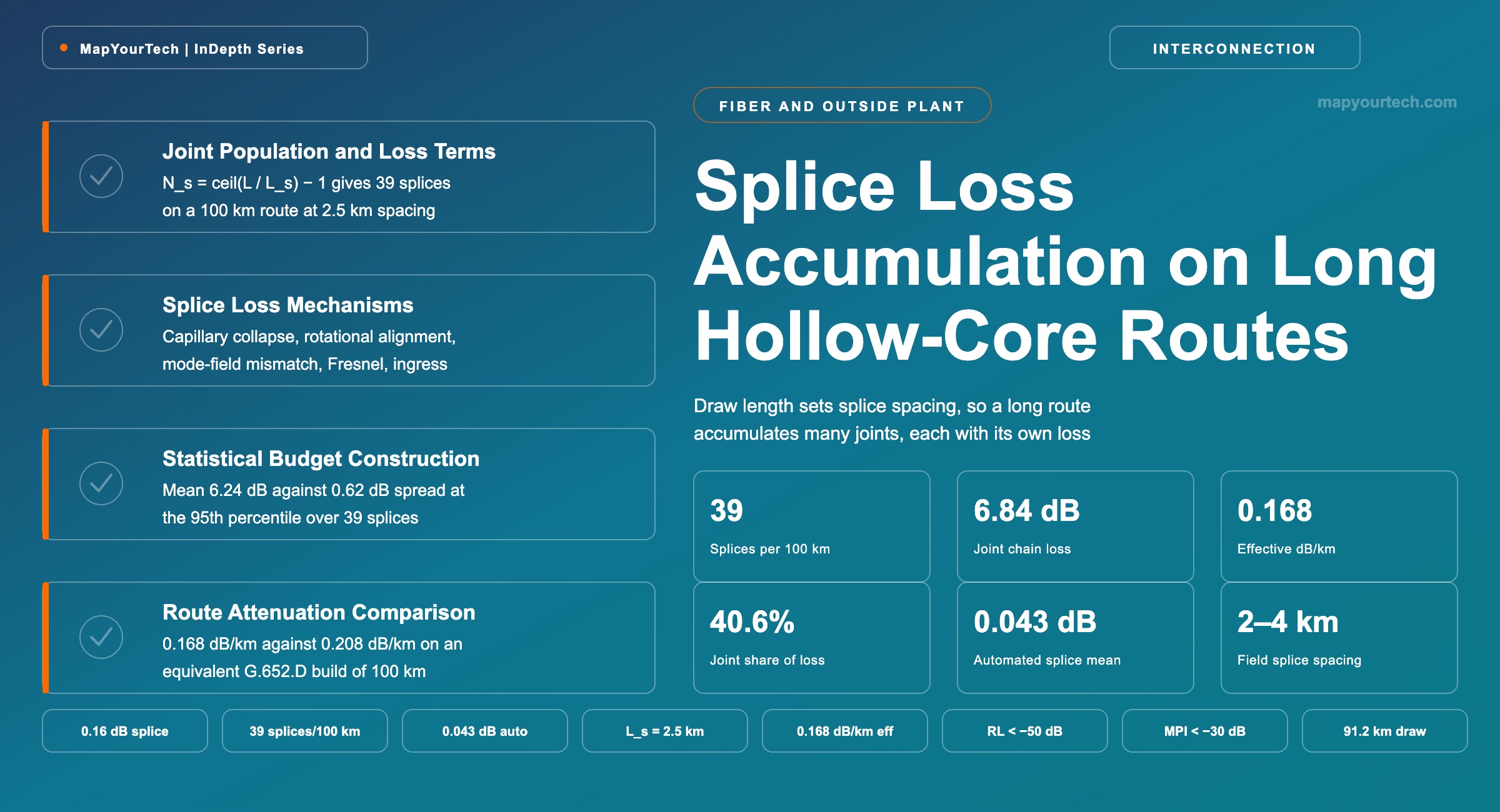
Draw length sets splice spacing, so a long route accumulates many joints, each with its own loss and reflectance — build the budget from splice statistics and adapter counts, not from a single best-case figure.
A splice loss is permanent; a connector loss is a maintenance decision.
What You Will Learn
- Define accumulated joint loss and splice spacing from first principles, and place every joint class on the route using Figure 1.
- Convert a qualified draw length into a joint population with N_s = ceil(L / L_s) − 1, giving 39 splices on a 100 km route at 2.5 km spacing.
- Build the joint term from splice statistics: 39 × 0.16 dB plus 2 × 0.30 dB = 6.84 dB, against 1.68 dB at the 0.043 dB automated mean.
- Quantify why the mean term dominates the tail, with the statistical margin at 0.62 dB against a mean of 6.24 dB in the design case of Section 5.
- Separate the five splice-loss mechanisms of Figure 2 into the two the process controls and the three the fiber pair fixes.
- Budget reflectance and multipath interference alongside insertion loss, working from −35 dB per-splice modal coupling and the −30 dB PAM4 threshold.
- Select the measurement stage that closes the budget, using the 0.32 dB against 0.11 dB divergence recorded in Figure 4.
- Compare the resulting 0.168 dB/km effective route attenuation against 0.208 dB/km on a G.652 route of the same length.
1. Introduction
A hollow-core fiber draw ends when the preform is exhausted or when the antiresonant membrane thickness drifts outside its tolerance, and the length reached before that happens propagates into every downstream number on the route. China Telecom Research Institute and Guangdong University of Technology place a splice roughly every 2–3 km in anti-resonant hollow-core fiber field trials (measured field practice, OFC 2026). VIAVI's monitoring guidance gives the same population as 2–4 km spacing and notes that usable optical time-domain reflectometer dynamic range at short pulse width therefore governs the instrument choice (vendor-published). At either figure, a 100 km route carries between 24 and 49 fusion splices before a single connector is counted.
Set that against the fiber the joints interrupt. Production hollow-core fiber now ships at 0.10–0.15 dB/km (vendor-published). Research-grade double-nested antiresonant fiber from the University of Southampton and Microsoft Azure Fiber measured 0.091 dB/km at 1550 nm and held below 0.1 dB/km across an 18 THz window (measured, Nature Photonics), and YOFC reported a record 0.04 dB/km at Mobile World Congress Barcelona 2026 (vendor-published). More than 1,200 km of hollow-core fiber is installed and carrying live Azure traffic (vendor-published), which is a deployment figure and not a loss measurement. Standard G.652.D fiber sits at 0.18–0.20 dB/km at 1550 nm in deployed cable (measured, typical field value). The distributed attenuation advantage is therefore close to a factor of two, which is the number that drives the business case and the number most published treatments stop at. The joint chain removes a large part of it.
Microsoft Azure reports a mean deployed splice loss of 0.16 dB across its hollow-core installation, with individual splices as low as 0.04 dB (vendor-published). Applied to 39 splices, the mean figure alone contributes 6.24 dB — more than half of the 10.00 dB the fiber itself contributes over 100 km at 0.10 dB/km. A budget built from the 0.04 dB best case would predict 1.56 dB for the same chain and understate the route by 4.68 dB, which is enough to reclassify a link from unamplified to amplified. A budget built from a 0.30 dB rework threshold would predict 11.70 dB and overstate it by 5.46 dB, which is enough to insert an amplifier site that the route does not need.
This article works one route: 100 km of hollow-core fiber, point-to-point, C-band, single fiber type, terminated on standard single-mode fiber at both ends. It defines the joint population from first principles, builds the loss budget from splice statistics rather than from any single figure, propagates reflectance and multipath interference alongside insertion loss, sets out which measurement stage each number may legitimately come from, and closes with the effective route attenuation compared against an equivalent G.652 build. Every figure carries its evidence class where it appears — standard-specified, measured, vendor-published, theoretical limit, or a design value chosen for this study so that a reader can substitute their own.
2. Splice Spacing and Accumulated Joint Loss Definitions
Accumulated joint loss is the sum of the discrete insertion losses contributed by every fusion splice and every fiber-type transition along one optical path, expressed in decibels and counted separately from the distributed attenuation of the fiber itself. Splice spacing is the length of contiguous cabled fiber between two adjacent joints, and follows from the qualified continuous draw length.
Read the Full Analysis with Premium
The remaining 88% of this article — the design numbers, trade-offs and field guidance — is part of MapYourTech Premium, along with the full premium library, courses and professional tools.
You May Also Like
-
Premium
-
August 27, 2026
-
Premium
-
August 27, 2026
-
Premium
-
August 27, 2026