
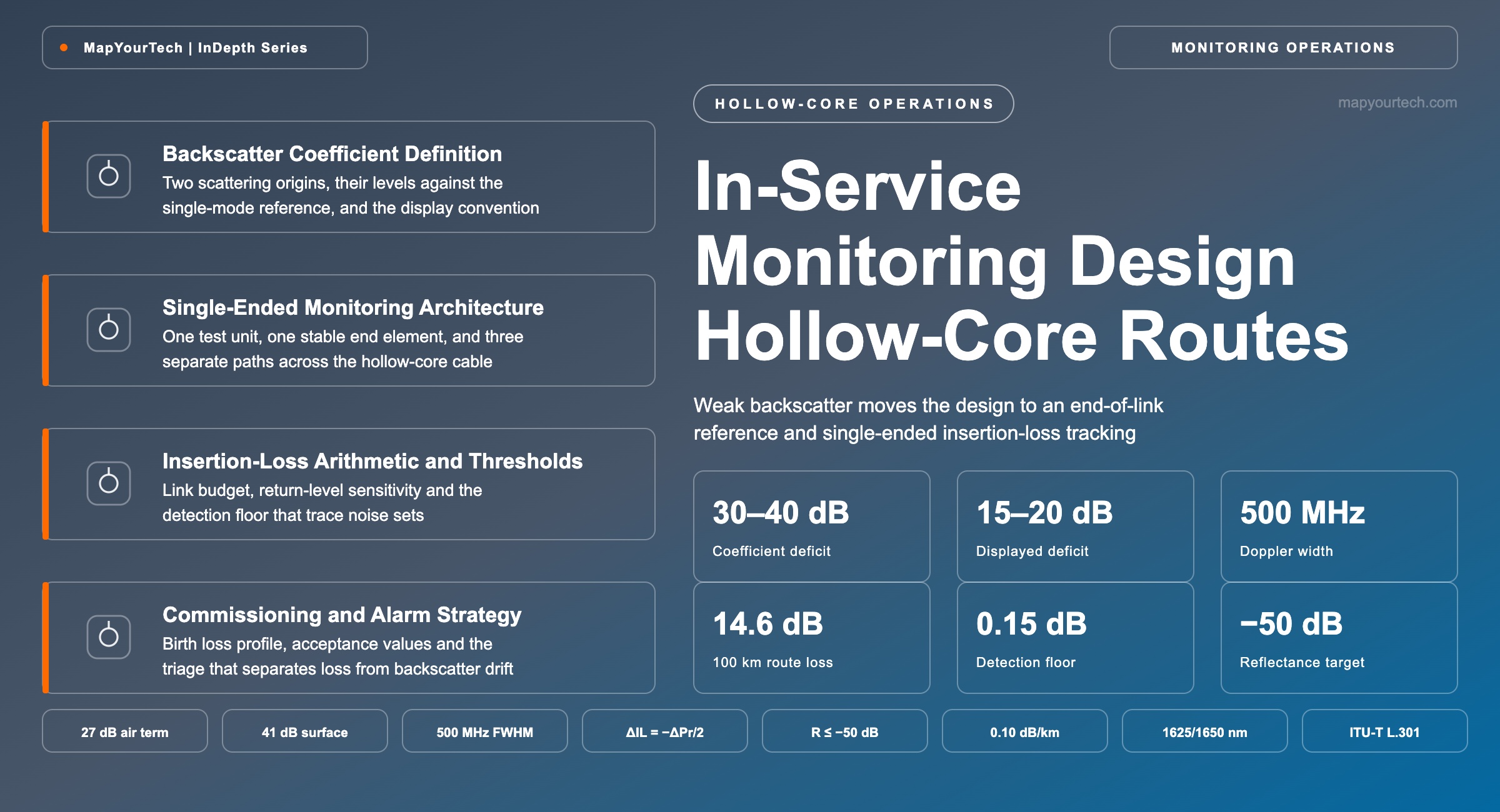
In-Service Monitoring Design for Hollow-Core Routes
Weak backscatter moves the monitoring design toward a stable end-of-link reference and single-ended insertion-loss tracking instead of trace-shape analysis — the architecture, the witness-fiber option and the alarm strategy.
A metric with no threshold is a number nobody acts on.
What You Will Learn
- Define the hollow-core backscatter coefficient from its two physical origins and derive the 15–20 dB displayed trace deficit from the 30–40 dB power deficit (Section 2, Fig. 1).
- Separate the backscatter coefficient, the displayed trace level and the instrument dynamic range, and state which of the three a pulse-width change moves (Section 2).
- Place a stable end element and read total insertion loss from its return level, using ΔIL = −ΔPr/2 rather than a fitted backscatter slope (Section 5).
- Build the four-layer monitoring model — witness fiber, link insertion loss, localization, on-demand diagnosis — and state what each layer cannot see (Section 4, Fig. 4).
- Quantify the 100 km worked route at 14.6 dB total insertion loss and set the 0.30 dB return-level alarm floor that follows from trace noise (Section 5).
- Select a monitoring wavelength against the anti-resonance window, the mode-field adapter bandwidth and the −50 dB/km multi-path interference plateau at 1625 nm (Section 4).
- Separate a real attenuation event from backscatter drift with a single bidirectional acquisition, and route each verdict to its own action (Section 7, Fig. 5).
- Set commissioning acceptance values for splice loss, transition reflectance and birth loss profile, and cross-check reflectometer readings against a power meter (Section 8, Table 4).
1. Introduction
A hollow-core span returns far less light to a reflectometer than the standard single-mode fiber running beside it in the same duct. Published reflectometry studies place the backscatter coefficient of anti-resonant hollow-core fiber roughly 30–40 dB below the single-mode Rayleigh level, and a coherent-detection measurement puts the glass-surface component about 41 dB below it (measured). Field test-equipment guidance reports the resulting trace level 14–20 dB below an equivalent single-mode measurement, and a second instrument supplier quotes approximately 15 dB (vendor-stated). The two sets of numbers are not in conflict, and Section 2 shows why: an optical power deficit appears on a reflectometer display at half its size, because the display halves the vertical scale so that fiber attenuation reads one-way. Every monitoring decision on a hollow-core route follows from that halved figure.
What the deficit removes is trace-shape analysis. On single-mode fiber an operations team reads the backscatter slope directly: a step at a splice, a change of gradient across a section, a bend signature developing over months. On hollow-core fiber the backscatter coefficient is not uniform along the fiber — it varies with microstructure and with the gas content and pressure inside the core — so the trace can change shape without the link losing a single decibel of budget (measured). An alarm policy built on trace shape therefore generates events with no transmission meaning, and an alarm stream with no transmission meaning is one an operations team learns to ignore.
What replaces it is narrower and more stable. A well-characterized reflective element at the far end of the link returns a known fraction of whatever reaches it, so its return level on each scan tracks twice the total insertion loss of the link. That reading needs one instrument at one end, needs no access to the far end after commissioning, and does not depend on the hollow-core backscatter signature at all. Around it sit three further layers: a witness fiber for cable integrity, an adaptive unidirectional baseline for localizing a change to a known splice position, and an on-demand bidirectional acquisition that decides whether an apparent change is real loss or backscatter drift.
The deployment context makes the question current rather than theoretical. Production hollow-core installations exceeded 1,200 km during 2025, with one hyperscaler stating a 15,000 km target, and deployed links now run to lengths on the order of a hundred kilometers at losses below 0.1 dB/km (vendor claim and reported deployment figures). The loss record stands at 0.04 dB/km (measured). No ITU-T G-series Recommendation covers hollow-core fiber — the G.652 to G.657 family describes solid-core designs — and ITU-T Study Group 15 is working toward a first technical report on the technology, with a national standards body having opened a test-methods project for hollow-core transmission characteristics (reported standards status). Monitoring practice therefore has to be built from the physics and from existing maintenance Recommendations rather than read off a fiber specification. That is what this article does: it defines the backscatter quantity, derives what a reflectometer can and cannot resolve on hollow-core fiber, builds the four-layer architecture, works the insertion-loss arithmetic through a 100 km route, and sets the alarm thresholds that follow from it. Readers new to the medium may want the physics of guidance in an air core and the reflectometry fundamentals first.
2. Backscatter Coefficient Definition and Component Terms
The backscatter coefficient is the fraction of launched optical power that a unit length of fiber returns toward the source, quoted in dB relative to the launched pulse or, in comparative work, in dB relative to the single-mode Rayleigh level. In hollow-core fiber the coefficient sums two independent physical terms: Rayleigh scattering from air molecules inside the core, and scattering from roughness frozen into the glass core wall.
Read the Full Analysis with Premium
The remaining 88% of this article — the design numbers, trade-offs and field guidance — is part of MapYourTech Premium, along with the full premium library, courses and professional tools.
You May Also Like
-
Premium
-
August 27, 2026
-
Premium
-
August 27, 2026
-
Premium
-
August 27, 2026