
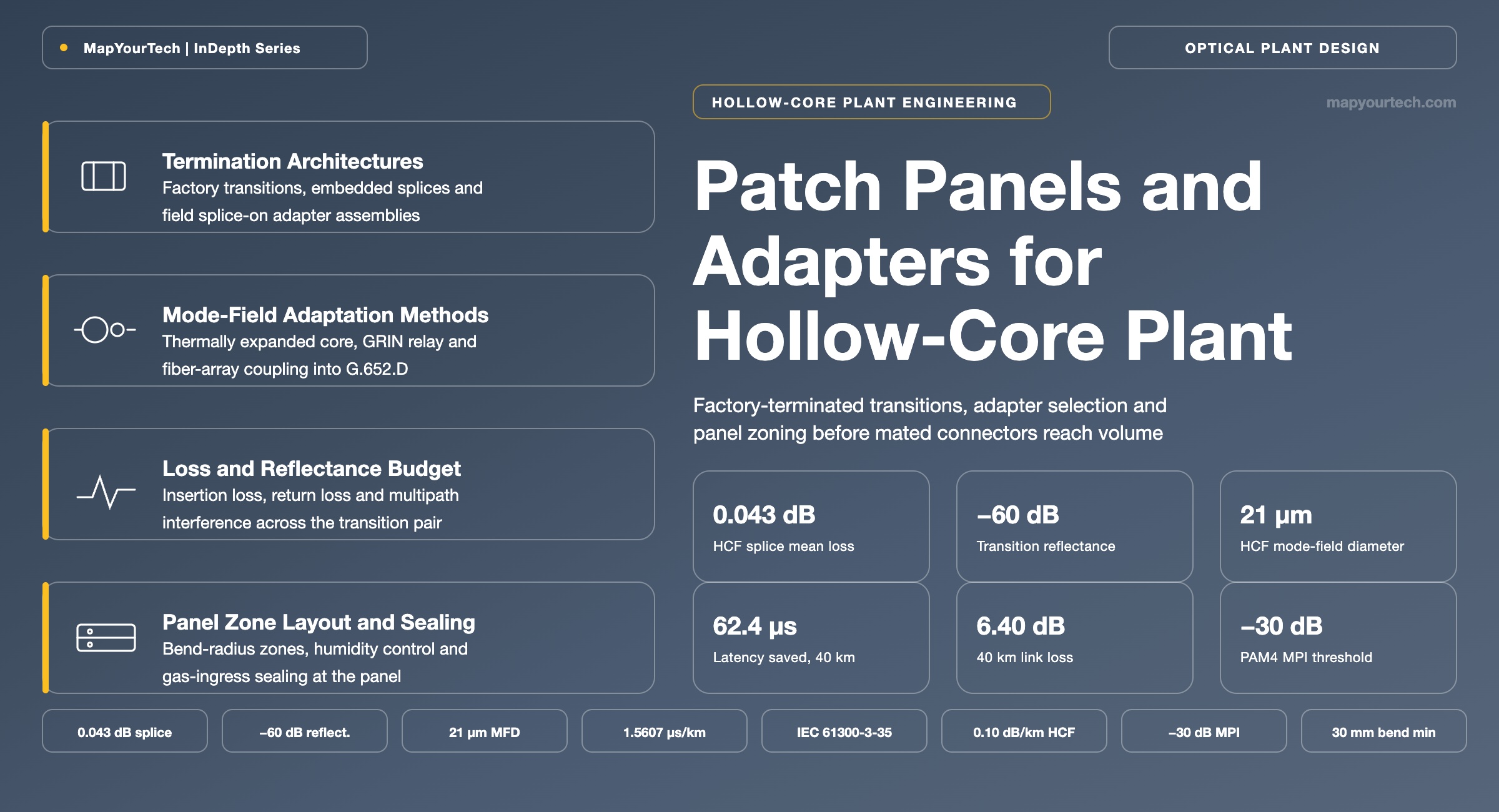
Patch Panel and Adapter Design for Hollow-Core Plant
Terminating air-guided fiber in a data-hall panel while commodity hollow-core connectors are still unavailable: adapter assemblies, transition loss and reflectance, zone layout, sealing, acceptance testing, and the migration path to a mated hollow-core interface.
A splice loss is permanent; a connector loss is a maintenance decision.
What You Will Learn
- Define the hollow-core to single-mode transition from its two figures of merit, and reproduce the 1.99 dB butt-joint loss and −14.7 dB reflectance of Figure 1 from the mode-overlap and Fresnel relations.
- Place the transition in one of the three architectures of Figure 2 and state what each costs in insertion loss, reflectance and field time.
- Select a mode-field adaptation method from Table 2 against a target of 0.08–0.15 dB insertion loss and reflectance below −60 dB.
- Build the 6.40 dB loss budget and 62.4 µs latency figure of the 40 km worked example, including the nanoseconds the panel tails add back at glass speed.
- Lay out the four panel zones of Figure 3 around a 30 mm in-panel bend radius and a 24-fiber cable entry.
- Apply the sealing and humidity rules that keep water absorption near 1364 nm and gas ingress out of the link, including the 40% relative-humidity ceiling for field work.
- Run the acceptance sequence of Figure 4 against a −50 dB install reflectance limit and record a birth loss profile for later comparison.
- Convert today's panel into a connectorized one without re-splicing the outside plant, using the four design choices of Section 12.
1. Introduction
A hollow-core cable arriving at a data-hall termination panel cannot be finished the way a G.652.D cable is. The fiber carrying the signal guides light in an air core roughly 21 µm across against 10.4 µm of mode-field diameter in standard single-mode fiber at 1550 nm (measured, published anti-resonant designs), it holds a slight internal underpressure that draws contaminants into the microstructure from any open end (measured, field-trial reports), and no ferrule geometry, alignment tolerance or optical interface has been standardized for it. Every hollow-core link carrying traffic today therefore ends in a solid-core connector, and the joint that converts one guidance mechanism into the other sits behind the panel's front face rather than on it.
That constraint is now a volume problem rather than a laboratory one. Microsoft reports more than 1,280 km of hollow-core fiber carrying production traffic with a 15,000 km build announced (vendor-published), Amazon Web Services is deploying hollow-core fiber to connect about ten data centers, principally for metro availability-zone interconnect (trade-press interview), and China Mobile's 20 km Shenzhen to Hong Kong commercial line runs at 0.085 dB/km average cable loss (vendor-published). On the cable side, Prysmian and Relativity Networks have manufactured a 10 mm cable carrying 24 hollow-core fibers and jetted it at up to 350 ft/min, about 107 m/min (vendor-published). Twenty-four fibers per cable means forty-eight transitions per point-to-point route, and each one is currently a hand-built assembly rather than a plug.
The economics reinforce the same point. Hollow-core fiber sells at roughly $5–10 per meter against $0.10 per meter for high-volume single-mode fiber (published market analysis), so a 5 km campus link carries about $25,000–50,000 of fiber cost (published cost model). Against that, cabled fiber accounts for only 5–10% of outside-plant deployment cost (published cost model), which puts termination labor, panel hardware and rework squarely inside the decision. A transition that has to be rebuilt in the field costs more than the fiber it joins.
This article covers the panel side of that plant: where the transition is made, what an adapter assembly contains, how loss and reflectance accumulate across it, how the panel is laid out and sealed, what acceptance testing has to prove, and what changes when a mated hollow-core interface reaches production. It assumes anti-resonant hollow-core fiber in C-band service at 1550 nm, and marks the places where photonic bandgap plant behaves differently. Readers new to the fiber itself will find the guidance mechanism covered in the MapYourTech article on the physics of light in air, and the deployment status in the readiness assessment for practical deployment.
2. Hollow-Core to Single-Mode Transition Definition and Component Terms
A hollow-core to single-mode transition is the joint that converts an air-guided fundamental mode into a glass-guided one. It contains a mode-field adapter that resizes the beam, a fusion joint that holds the two fibers together, and a treated end face that controls reflection. Its two figures of merit are insertion loss in dB and reflectance in dB, and a design that reports only the first is describing half the joint.
2.1 Distinctions From the Adjacent Quantities
Three pairs of terms get conflated in hollow-core plant documentation, and each pair carries a different number. Transition loss is the one-way insertion loss of the complete hollow-core to single-mode joint, adapter included, and lands between 0.08 dB and 0.15 dB in published demonstrations (measured). Mated-pair connector loss is the loss of two solid-core ferrules meeting in an adapter sleeve, bounded at 0.25 dB maximum for IEC 61753 Grade B and 0.50 dB for Grade C (standard-specified); the panel carries several of these and none of them touch the hollow core. Fusion splice loss is the loss of a hollow-core to hollow-core joint, at 0.043 dB mean across thirty automated field-representative trials (measured, OFC 2026).
Read the Full Analysis with Premium
The remaining 88% of this article — the design numbers, trade-offs and field guidance — is part of MapYourTech Premium, along with the full premium library, courses and professional tools.
You May Also Like
-
Premium
-
August 27, 2026
-
Premium
-
August 27, 2026
-
Premium
-
August 27, 2026