Fundamentals of Noise Figure in Optical Amplifiers

Technical 14 Mins Read

Fundamentals of Noise Figure in Optical Amplifiers

Noise figure (NF) is a critical parameter in optical amplifiers that quantifies the degradation of signal-to-noise ratio during amplification. In multi-span optical networks, the accumulated noise from cascaded amplifiers ultimately determines system reach, capacity, and performance.

While amplifiers provide the necessary gain to overcome fiber losses, they inevitably add amplified spontaneous emission (ASE) noise to the signal. The noise contribution from each amplifier accumulates along the transmission path, with early-stage amplifiers having the most significant impact on the end-to-end system performance.

Understanding the noise behavior in cascaded amplifier chains is fundamental to optical network design. This article explores noise figure fundamentals, calculation methods, and the cumulative effects in multi-span networks, providing practical design guidelines for optimizing system performance.

Definition and Physical Meaning

Noise figure is defined as the ratio of the input signal-to-noise ratio (SNR) to the output SNR of an amplifier, expressed in decibels (dB):

NF = 10 log₁₀(SNR_in / SNR_out) dB

Alternatively, it can be expressed using the noise factor F (linear scale):

NF = 10 log₁₀(F) dB

In optical amplifiers, the primary noise source is amplified spontaneous emission (ASE), which originates from spontaneous transitions in the excited gain medium. Instead of being stimulated by the input signal, these transitions occur randomly and produce photons with random phase and direction.

Quantum Limit and Physical Interpretation

Even a theoretically perfect amplifier has a quantum-limited minimum noise figure of 3dB. This fundamental limit exists because the amplification process inherently introduces at least half a photon of noise per mode.

The noise figure is related to several physical parameters:

Spontaneous Emission Factor (nsp): Represents the quality of population inversion in the active medium
Population Inversion: The ratio of atoms in excited states versus ground states
Quantum Efficiency: How efficiently pump power creates population inversion

NF = 2·nsp·(1-1/G)

As gain (G) becomes large, this approaches: NF = 2·nsp, with a theoretical minimum of 3dB when nsp = 1.

Factors Affecting Noise Figure

Gain and Population Inversion

The population inversion level directly affects the noise figure. Higher inversion leads to lower ASE and therefore lower noise figure. Key relationships include:

Gain Level: Higher gain typically results in better inversion and lower NF up to a saturation point
Pump Power: Increased pump power improves inversion up to a saturation level
Gain Medium Length: Longer gain medium increases available gain but can increase NF if inversion is not maintained throughout

Input Power Dependence

Noise figure varies with input signal power:

At very low input powers, the gain can be higher but the effective NF may increase due to insufficient saturation
At high input powers, gain saturation occurs, leading to a higher effective NF
The optimal input power range for lowest NF is typically 10-15dB below the saturation input power

Wavelength Dependence

Noise figure typically varies across the operating wavelength band:

The wavelength dependence follows the gain spectrum of the amplifier
In typical optical amplifiers, NF is often lowest near the peak gain wavelength
Edge wavelengths generally experience higher NF due to lower inversion and gain
This wavelength dependence can impact system design, especially for wideband applications

Temperature Effects

Temperature significantly impacts noise figure performance:

Higher temperatures typically increase NF due to reduced population inversion efficiency
Temperature-dependent cross-sections in the gain medium affect both gain and noise performance
Thermal management is critical for maintaining consistent NF performance, especially in high-power amplifiers

EDFA Specifications

In optical networks, various EDFA designs are available with specific noise figure performance characteristics:

Application	Typical NF Range	Typical Gain Range
Metro access	6.0-7.0dB	12-21dB
Metro/regional	5.5-6.5dB	14-22dB
Regional with mid-stage access	5.5-7.5dB	15-28dB
Long-haul with mid-stage access	5.0-7.0dB	25-37dB
Regional single-stage	5.0-6.0dB	15-28dB
Long-haul single-stage	5.0-6.0dB	25-37dB
Ultra-short span booster	15.0-17.0dB	5-7dB

Temperature Sensitivity

Noise figure is temperature sensitive, with performance typically degrading at higher temperatures due to:

Reduced pump efficiency
Changes in population inversion
Increased thermal noise contributions

Most optical amplifiers are designed to operate in accordance with standard telecom environmental specifications like ETS 300 019-1-3 Class 3.1E for environmental endurance.

Cascaded Amplifiers and Noise Accumulation

In optical networks, signals typically pass through multiple amplifiers as they traverse through fiber spans. Understanding how noise accumulates in these multi-span systems is critical for designing networks that meet performance requirements.

Friis' Formula and Cascaded Amplifier Systems

The noise accumulation in a chain of optical amplifiers follows Friis' formula, which was originally developed for electronic amplifiers but applies equally to optical systems:

F_total = F₁ + (F₂-1)/G₁ + (F₃-1)/(G₁·G₂) + ... + (F_n-1)/(G₁·G₂···G_n-1)

Where:

F_total is the total noise factor (linear, not in dB)
F_i is the noise factor of the i-th amplifier
G_i is the gain (linear) of the i-th amplifier

In optical systems, this formula must account for span losses between amplifiers:

F_total = F₁ + (L₁·F₂-1)/G₁ + (L₁·L₂·F₃-1)/(G₁·G₂) + ...

Where L_i represents the span loss (linear) between amplifiers i and i+1.

Key Insights from Friis' Formula

The most significant insight from Friis' formula is that the first amplifier has the most substantial impact on the overall noise performance. Each subsequent amplifier's noise contribution is reduced by the gain of all preceding amplifiers.

Practical implications include:

Always use the lowest noise figure amplifier at the beginning of a chain
The impact of noise figure improvements diminishes for amplifiers later in the chain
Pre-amplifiers are more critical for noise performance than boosters
Mid-stage components (like DCFs) should have minimal loss to preserve good noise performance

OSNR Evolution in Multi-span Systems

The optical signal-to-noise ratio (OSNR) evolution through a multi-span system can be approximated by:

OSNR_dB ≈ P_launch - α·L - NF - 10·log₁₀(N) - 10·log₁₀(B_ref) + 58

Where:

P_launch is the launch power per channel (dBm)
α is the fiber attenuation coefficient (dB/km)
L is the span length (km)
NF is the amplifier noise figure (dB)
N is the number of spans
B_ref is the reference bandwidth for OSNR measurement (typically 0.1nm)
58 is a constant that accounts for physical constants (h𝜈)

The key insight from this equation is that OSNR degrades by 3dB each time the number of spans doubles (10·log₁₀(N) term). This creates a fundamental limit to transmission distance in amplified systems.

Practical Example: OSNR Calculation in a Multi-span System

Consider a 10-span system with the following parameters:

Launch power: +1dBm per channel
Span length: 80km
Fiber loss: 0.2dB/km (total span loss = 16dB)
Amplifier gain: 16dB (exactly compensating span loss)
Amplifier noise figure: 5dB
Reference bandwidth: 0.1nm (~12.5GHz at 1550nm)

Step 1: Calculate the OSNR for a single span:

OSNR_1-span = +1 - 16 - 5 - 10·log₁₀(1) - 10·log₁₀(12.5) + 58

= +1 - 16 - 5 - 0 - 11 + 58 = 27dB

Step 2: Calculate the OSNR degradation due to multiple spans:

OSNR degradation = 10·log₁₀(N) = 10·log₁₀(10) = 10dB

Step 3: Calculate the final OSNR:

OSNR_10-spans = OSNR_1-span - 10·log₁₀(N) = 27 - 10 = 17dB

With a typical OSNR requirement of 12-15dB for modern coherent transmission formats, this system has adequate margin for reliable operation. However, extending to 20 spans would reduce OSNR by another 3dB to 14dB, approaching the limit for reliable operation.

Multi-Stage Amplifier Design

Based on the principles of Friis' formula, multi-stage amplifiers with optimal noise performance typically follow a design where:

Key design principles include:

Low-Noise First Stage: The first stage should be optimized for low noise figure, even at the expense of output power capability
Power-Optimized Second Stage: The second stage can focus on power handling and efficiency once the SNR has been established by the first stage
Minimal Mid-Stage Loss: Any passive components (filters, isolators, etc.) between stages should have minimal insertion loss to avoid degrading the noise performance

EDFA Models and Cascaded Performance

Various types of optical amplifiers are designed with cascaded performance in mind:

Type	Mid-Stage Features	Design Optimization
Variable gain with mid-stage access	Mid-stage access for DCF	Optimized for regional networks
High-gain variable gain with mid-stage access	Mid-stage access for DCF	Optimized for high-gain applications
Variable gain with mid-stage access and C/T filters	Mid-stage access for DCF	Optimized for high-power applications with OSC handling

Typical mid-stage dispersion compensation fiber (DCF) parameters tracked in optical networks include dispersion value, PMD, and tilt, which are critical for maintaining overall system performance.

Automatic Laser Shutdown (ALS) and Safety

In high-power multi-span systems, safety mechanisms like Automatic Laser Shutdown (ALS) are implemented to prevent hazardous conditions during fiber breaks or disconnections:

ALS triggers when LOS (Loss Of Signal) is detected on a line port
During ALS, EDFAs are disabled except for periodic 30-second probing intervals at reduced power (20dBm)
Normal operation resumes only after signal restoration for at least 40 seconds

Modern optical amplifiers feature ALS functionality with configurable parameters to ensure both optimal performance and safety in cascaded environments.

Network Applications and Optimization Strategies for Optical Amplifiers

Different segments of optical networks have varying requirements for noise figure performance based on their application, reach requirements, and economic considerations.

Network Segment Requirements

Access Networks

Access networks are generally tolerant of higher noise figures (6-7dB) because:

They involve fewer amplifiers in cascade
They often operate with higher channel powers
Transmission distances are relatively short
Cost sensitivity is higher than performance optimization

Metro/Regional Networks

Metro and regional networks require balanced NF performance (5-6dB) with:

Good dynamic range to handle varying traffic patterns
Flexibility to support different node configurations
Moderate reach capabilities (typically 4-10 spans)
Reasonable cost-performance trade-offs

Long-haul Networks

Long-haul and submarine networks demand optimized low-NF designs (4-5dB) due to:

Large number of amplifiers in cascade (often 10-20+)
Need to maximize reach without electrical regeneration
Requirement to support advanced modulation formats
Justification for premium components due to overall system economics

Economic Implications of Noise Figure

Improving noise figure comes with cost implications that must be carefully evaluated:

NF Improvement	Typical Cost Increase	Performance Benefit	Economic Justification
6.0dB → 5.5dB	+5-10%	~10% reach increase	Generally cost-effective
5.5dB → 5.0dB	+10-15%	~10% reach increase	Often justified for long-haul
5.0dB → 4.5dB	+15-25%	~10% reach increase	Specialty applications only
4.5dB → 4.0dB	+30-50%	~10% reach increase	Rarely justified economically

The economic tradeoffs include:

Capital vs. Operating Expenses: Higher-quality, lower-NF amplifiers cost more initially but may reduce the need for additional amplifier sites and regeneration points
Upgrade Paths: Better NF provides margin for future capacity upgrades with more advanced modulation formats
Lifecycle Considerations: Premium amplifiers may maintain better performance over their operational lifetime, delaying replacement needs
System Capacity: Improved NF can enable higher capacity through better OSNR margin, often at lower cost than adding new fiber routes

Operational Optimization Strategies

For system operators using EDFAs, several practical optimization strategies can help maximize performance:

1. Gain Optimization

Modern optical amplifiers support different operation modes with specific gain management approaches:

Automatic Mode: Maintains output power per channel based on saturation power and maximum channel count settings
Semi-automatic Mode: Maintains a fixed output power per channel
Constant Gain Mode: Maintains a fixed gain regardless of input power variations
Automatic Power Control (APC) Mode: Provides automatic power control for specialized applications
Automatic Current Control (ACC) Mode: Provides precise pump current control for specialized applications

Advanced amplifiers implement specific algorithms for gain control that include careful monitoring of required gain versus actual gain, with alarms for out-of-range or out-of-margin conditions.

2. Tilt Management

Spectral tilt management is crucial for maintaining consistent OSNR across all channels:

Modern EDFAs automatically adjust tilt to compensate for fiber and component tilt
SRS (Stimulated Raman Scattering) tilt compensation is included for high-power systems
Built-in tilt values are stored in amplifier memory and used as reference points
For ultra-short span boosters and extended C-band amplifiers, specialized tilt algorithms account for fiber type

3. Temperature Control

Optical amplifiers typically specify operational temperature ranges in accordance with telecom standards like ETS 300 019-1-3 Class 3.1E, emphasizing the importance of controlling environmental conditions to maintain optimal performance.

4. Fiber Plant Optimization

Several fiber plant parameters impact noise figure performance:

Span Loss: Monitored and alarmed when outside expected range
Mid-stage Loss: For dual-stage amplifiers, carefully managed for optimal performance
Transmission Fiber Type: Configuration option that affects SRS tilt compensation
DCF Parameters: Dispersion, PMD, and tilt tracked in network control protocols

Noise Figure Design Guidelines

Place Highest Quality First: Always use the lowest noise figure amplifiers at the beginning of the chain where they have the most impact
Budget Wisely: Budget 0.5-1.0dB extra margin for each amplifier to account for aging and temperature variations over the system lifetime
Consider Total Cost: Evaluate the total cost impact of NF improvements, including reduced regeneration needs and extended reach capabilities
Monitor Trends: Establish baseline NF measurements and monitor for gradual degradation that might indicate pump laser aging
Balance Requirements: Balance NF with other parameters like output power, gain flatness, and dynamic range based on specific application needs
Test Under Load: Validate NF performance under realistic channel loading conditions, not just with a single test wavelength

Future Trends in Noise Figure Technology

Emerging technologies for noise figure optimization include:

AI-Driven Optimization: Machine learning algorithms that dynamically adjust amplifier parameters based on real-time network conditions
Advanced Material Science: New dopant materials and glass compositions that enable better population inversion and reduced spontaneous emission
Integrated Photonics: Silicon photonics and other integrated platforms that combine amplification with filtering and control functions
Quantum-Enhanced Amplification: Phase-sensitive amplification and other quantum approaches that can theoretically break the 3dB quantum noise limit
Distributed Intelligence: Network-wide optimization that coordinates multiple amplifiers for global noise minimization

EDFA Implementation Examples

Metro Network Design

A typical metro network implementation might include:

Terminal nodes using fixed-gain boosters and pre-amplifiers
FOADM nodes using low-gain pre-amplifiers
Flexible OADM nodes employing medium-gain boosters

Regional Network Design

For regional networks, typical designs include:

Terminal nodes with AWG Mux/DeMux and EDFAs for amplification
Modern terminals with WSS for automatic equalization
ROADM nodes employing pre-amplifiers with mid-stage access for DCF compensation and boosters
In-line amplifier nodes (ILAN) using EDFAs to compensate for transmission fiber and DCF loss

Specialized Applications

Some specialized EDFA designs address unique requirements:

Ultra-short span boosters: Very high output power (26dBm) with narrow gain range (5-7dB)
High-power pre-amps: For ROADM applications with specialized eye-safety verification process
Pluggable EDFAs: For applications requiring compact, modular amplification in form factors like CFP2

Conclusion

Noise figure is a fundamental parameter that sets ultimate performance limits for optical amplifier systems. Modern EDFA families demonstrate a comprehensive approach to addressing various network requirements with optimized designs for different applications.

Key takeaways include:

Noise figure quantifies an amplifier's SNR degradation, with a quantum-limited minimum of 3dB
In cascaded configurations, noise accumulates according to Friis' formula, with early-stage amplifiers having the most significant impact
Network operators can optimize NF through proper pump power settings, gain optimization, temperature control, and careful wavelength planning
Multi-stage designs with low-NF first stages offer the best overall performance for critical applications
Economic considerations must balance the additional cost of lower-NF amplifiers against improved system reach and capacity

The evolution of EDFA technology reflects the ongoing refinement of noise figure optimization techniques, with newer designs and features continually addressing the evolving requirements of optical networks.

ZR vs. ZR+: Navigating the Evolution of Coherent Optical Standards

Technical 4 Mins Read

In this ever-evolving landscape of optical networking, the development of coherent optical standards, such as 400G ZR and ZR+, represents a significant leap forward in addressing the insatiable demand for bandwidth, efficiency, and scalability in data centers and network infrastructure. This technical blog delves into the nuances of these standards, comparing their features, applications, and how they are shaping the future of high-capacity networking. ZR stands for “Ze Best Range” and ZR+ is reach “Ze Best Range plus”

Introduction to 400G ZR

The 400G ZR standard, defined by the Optical Internetworking Forum (OIF), is a pivotal development in the realm of optical networking, setting the stage for the next generation of data transmission over optical fiber’s. It is designed to facilitate the transfer of 400 Gigabit Ethernet over single-mode fiber across distances of up to 120 kilometers without the need for signal amplification or regeneration. This is achieved through the use of advanced modulation techniques like DP-16QAM and state-of-the-art forward error correction (FEC).

Key features of 400G ZR include:

High Capacity: Supports the transmission of 400 Gbps using a single wavelength.
Compact Form-Factor: Integrates into QSFP-DD and OSFP modules, aligning with industry standards for data center equipment.
Cost Efficiency: Reduces the need for external transponders and simplifies network architecture, lowering both CAPEX and OPEX.

Emergence of 400G ZR+

Building upon the foundation set by 400G ZR, the 400G ZR+ standard extends the capabilities of its predecessor by increasing the transmission reach and introducing flexibility in modulation schemes to cater to a broader range of network topologies and distances. The OpenZR+ MSA has been instrumental in this expansion, promoting interoperability and open standards in coherent optics.

Key enhancements in 400G ZR+ include:

Extended Reach: With advanced FEC and modulation, ZR+ can support links up to 2,000 km, making it suitable for longer metro, regional, and even long-haul deployments.
Versatile Modulation: Offers multiple configuration options (e.g., DP-16QAM, DP-8QAM, DP-QPSK), enabling operators to balance speed, reach, and optical performance.
Improved Power Efficiency: Despite its extended capabilities, ZR+ maintains a focus on energy efficiency, crucial for reducing the environmental impact of expanding network infrastructures.

ZR vs. ZR+: A Comparative Analysis

Feature.	400G ZR	400G ZR+
Reach	Up to 120 km	Up to 2,000 km
Modulation	DP-16QAM	DP-16QAM, DP-8QAM, DP-QPSK
Form Factor	QSFP-DD, OSFP	QSFP-DD, OSFP
Application	Data center interconnects	Metro, regional, long-haul

Adding few more interesting table for readers

Based on application

Product	Reach	Client Formats	Data Rate & Modulation	Wavelength	Tx Power	Connector	Fiber	Interoperability	Application
800G ZR+	4000 km+	100GbE 200GbE 400GbE 800GbE	800G Interop PCS 600G PCS 400G PCS	1528.58 to 1567.34	>+1 dBm (with TOF)	LC	SMF	OpenROADM interoperable PCS	Ideal for metro/regional Ethernet data center and service provider network interconnects
800ZR	120 km	100GbE 200GbE 400GbE	800G 16QAM 600G PCS 400G Interop QPSK/16QAM PCS	1528.58 to 1567.34	-11 dBm to -2 dBm	LC	SMF	OIF 800ZR OpenROADM Interop PCS OpenZR+	Ideal for amplified single-span data center interconnect applications
400G Ultra Long Haul	4000 km+	100GbE 200GbE 400GbE	400G Interoperable QPSK/16QAM PCS	1528.58 to 1567.34	>+1 dBm (with TOF)	LC	SMF	OpenROADM Interop PCS	Ideal for long haul and ultra-long haul service provider ROADM network applications
Bright 400ZR+	4000 km+	100GbE 200GbE 400GbE OTUCn OTU4	400G 16QAM 300G 8QAM 200G/100G QPSK	1528.58 to 1567.34	>+1 dBm (with TOF)	LC	SMF	OpenZR+ OpenROADM	Ideal for metro/regional and service provider ROADM network applications
400ZR	120 km	100GbE 200GbE 400GbE	400G 16QAM	1528.58 to 1567.34	>-10 dBm	LC	SMF	OIF 400ZR	Ideal for amplified single span data center interconnect applications
OpenZR+	4000 km+	100GbE 200GbE 400GbE	400G 16QAM 300G 8QAM 200G/100G QPSK	1528.58 to 1567.34	>-10 dBm	LC	SMF	OpenZR+ OpenROADM	Ideal for metro/regional Ethernet data center and service provider network interconnects
400G ER1	45 km	100GbE 400GbE	400G 16QAM	Fixed C to band	>12.5 dB Link Budget	LC	SMF	OIF 400ZR application code 0x02 OpenZR+	Ideal for unamplified point-to-point links

*TOF: Tunable Optical Filter

The Future Outlook

The advent of 400G ZR and ZR+ is not just a technical upgrade; it’s a paradigm shift in how we approach optical networking. With these technologies, network operators can now deploy more flexible, efficient, and scalable networks, ready to meet the future demands of data transmission.

Moreover, the ongoing development and expected introduction of XR optics highlight the industry’s commitment to pushing the boundaries of what’s possible in optical networking. XR optics, with its promise of multipoint capabilities and aggregation of lower-speed interfaces, signifies the next frontier in coherent optical technology.

Reference

Acacia Introduces 800ZR and 800G ZR+ with Interoperable PCS in QSFP-DD and OSFP

Optical Amplifiers Insight

Standards 8 Mins Read

Optical Amplifiers (OAs) are key parts of today’s communication world. They help send data under the sea, land and even in space .In fact it is used in all electronic and telecommunications industry which has allowed human being develop and use gadgets and machines in daily routine.Due to OAs only; we are able to transmit data over a distance of few 100s too 1000s of kilometers.

Classification of OA Devices

Optical Amplifiers, integral in managing signal strength in fiber optics, are categorized based on their technology and application. These categories, as defined in ITU-T G.661, include Power Amplifiers (PAs), Pre-amplifiers, Line Amplifiers, OA Transmitter Subsystems (OATs), OA Receiver Subsystems (OARs), and Distributed Amplifiers.

Scheme of insertion of an OA device

Power Amplifiers (PAs): Positioned after the optical transmitter, PAs boost the signal power level. They are known for their high saturation power, making them ideal for strengthening outgoing signals.
Pre-amplifiers: These are used before an optical receiver to enhance its sensitivity. Characterized by very low noise, they are crucial in improving signal reception.
Line Amplifiers: Placed between passive fiber sections, Line Amplifiers are low noise OAs that extend the distance covered before signal regeneration is needed. They are particularly useful in point-multipoint connections in optical access networks.
OA Transmitter Subsystems (OATs): An OAT integrates a power amplifier with an optical transmitter, resulting in a higher power transmitter.
OA Receiver Subsystems (OARs): In OARs, a pre-amplifier is combined with an optical receiver, enhancing the receiver’s sensitivity.
Distributed Amplifiers: These amplifiers, such as those using Raman pumping, provide amplification over an extended length of the optical fiber, distributing amplification across the transmission span.

Applications and Configurations

The application of these OA devices can vary. For instance, a Power Amplifier (PA) might include an optical filter to minimize noise or separate signals in multiwavelength applications. The configurations can range from simple setups like Tx + PA + Rx to more complex arrangements like Tx + BA + LA + PA + Rx, as illustrated in the various schematics provided in the IEC standards.

Building upon the foundational knowledge of Optical Amplifiers (OAs), it’s essential to understand the practical configurations of these devices in optical networks. According to the definitions of Booster Amplifiers (BAs), Pre-amplifiers (PAs), and Line Amplifiers (LAs), and referencing Figure 1 from the IEC standards, we can explore various OA device applications and their configurations. These setups illustrate how OAs are integrated into optical communication systems, each serving a unique purpose in enhancing signal integrity and network performance.

Tx + BA + Rx Configuration: This setup involves a transmitter (Tx), followed by a Booster Amplifier (BA), and then a receiver (Rx). The BA is used right after the transmitter to increase the signal power before it enters the long stretch of the fiber. This configuration is particularly useful in long-haul communication systems where maintaining a strong signal over vast distances is crucial.
Tx + PA + Rx Configuration: Here, the system comprises a transmitter, followed by a Pre-amplifier (PA), and then a receiver. The PA is positioned close to the receiver to improve its sensitivity and to amplify the weakened incoming signal. This setup is ideal for scenarios where the incoming signal strength is low, and enhanced detection is required.
Tx + LA + Rx Configuration: In this configuration, a Line Amplifier (LA) is placed between the transmitter and receiver. The LA’s role is to amplify the signal partway through the transmission path, effectively extending the reach of the communication link. This setup is common in both long-haul and regional networks.
Tx + BA + PA + Rx Configuration: This more complex setup involves both a BA and a PA, with the BA placed after the transmitter and the PA before the receiver. This combination allows for both an initial boost in signal strength and a final amplification to enhance receiver sensitivity, making it suitable for extremely long-distance transmissions or when signals pass through multiple network segments.
Tx + BA + LA + Rx Configuration: Combining a BA and an LA provides a powerful solution for extended reach. The BA boosts the signal post-transmission, and the LA offers additional amplification along the transmission path. This configuration is particularly effective in long-haul networks with significant attenuation.
Tx + LA + PA + Rx Configuration: Here, the LA is used for mid-path amplification, while the PA is employed near the receiver. This setup ensures that the signal is sufficiently amplified both during transmission and before reception, which is vital in networks with long spans and higher signal loss.
Tx + BA + LA + PA + Rx Configuration: This comprehensive setup includes a BA, an LA, and a PA, offering a robust solution for maintaining signal integrity across very long distances and complex network architectures. The BA boosts the initial signal strength, the LA provides necessary mid-path amplification, and the PA ensures that the receiver can effectively detect the signal.

Characteristics of Optical Amplifiers

Each type of OA has specific characteristics that define its performance in different applications, whether single-channel or multichannel. These characteristics include input and output power ranges, wavelength bands, noise figures, reflectance, and maximum tolerable reflectance at input and output, among others.

For instance, in single-channel applications, a Power Amplifier’s characteristics would include an input power range, output power range, power wavelength band, and signal-spontaneous noise figure. In contrast, for multichannel applications, additional parameters like channel allocation, channel input and output power ranges, and channel signal-spontaneous noise figure become relevant.

Optically Amplified Transmitters and Receivers

In the realm of OA subsystems like OATs and OARs, the focus shifts to parameters like bit rate, application code, operating signal wavelength range, and output power range for transmitters, and sensitivity, overload, and bit error ratio for receivers. These parameters are critical in defining the performance and suitability of these subsystems for specific applications.

Understanding Through Practical Examples

To illustrate, consider a scenario in a long-distance fiber optic communication system. Here, a Line Amplifier might be employed to extend the transmission distance. This amplifier would need to have a low noise figure to minimize signal degradation and a high saturation output power to ensure the signal remains strong over long distances. The specific values for these parameters would depend on the system’s requirements, such as the total transmission distance and the number of channels being used.

Advanced Applications of Optical Amplifiers

Long-Haul Communication: In long-haul fiber optic networks, Line Amplifiers (LAs) play a critical role. They are strategically placed at intervals to compensate for signal loss. For example, an LA with a high saturation output power of around +17 dBm and a low noise figure, typically less than 5 dB, can significantly extend the reach of the communication link without the need for electronic regeneration.
Submarine Cables: Submarine communication cables, spanning thousands of kilometers, heavily rely on Distributed Amplifiers, like Raman amplifiers. These amplifiers uniquely boost the signal directly within the fiber, offering a more distributed amplification approach, which is crucial for such extensive undersea networks.
Metropolitan Area Networks: In shorter, more congested networks like those in metropolitan areas, a combination of Booster Amplifiers (BAs) and Pre-amplifiers can be used. A BA, with an output power range of up to +23 dBm, can effectively launch a strong signal into the network, while a Pre-amplifier at the receiving end, with a very low noise figure (as low as 4 dB), enhances the receiver’s sensitivity to weak signals.
Optical Add-Drop Multiplexers (OADMs): In systems using OADMs for channel multiplexing and demultiplexing, Line Amplifiers help in maintaining signal strength across the channels. The ability to handle multiple channels, each potentially with different power levels, is crucial. Here, the channel addition/removal (steady-state) gain response and transient gain response become significant parameters.

Technological Innovations and Challenges

The development of OA technologies is not without challenges. One of the primary concerns is managing the noise, especially in systems with multiple amplifiers. Each amplification stage adds some noise, quantified by the signal-spontaneous noise figure, which can accumulate and degrade the overall signal quality.

Another challenge is the management of Polarization Mode Dispersion (PMD) in Line Amplifiers. PMD can cause different light polarizations to travel at slightly different speeds, leading to signal distortion. Modern LAs are designed to minimize PMD, a critical parameter in high-speed networks.

Future of Optical Amplifiers in Industry

The future of OAs is closely tied to the advancements in fiber optic technology. As data demands continue to skyrocket, the need for more efficient, higher-capacity networks grows. Optical Amplifiers will continue to evolve, with research focusing on higher power outputs, broader wavelength ranges, and more sophisticated noise management techniques.

Innovations like hybrid amplification techniques, combining the benefits of Raman and Erbium-Doped Fiber Amplifiers (EDFAs), are on the horizon. These hybrid systems aim to provide higher performance, especially in terms of power efficiency and noise reduction.

References

ITU-T :https://www.itu.int/en/ITU-T/Pages/default.aspx

Image :https://www.chinacablesbuy.com/guide-to-optical-amplifier.html

Noise Concatenation in Optical Amplifier Chains

Standards 4 Mins Read

Optical networks are the backbone of the internet, carrying vast amounts of data over great distances at the speed of light. However, maintaining signal quality over long fiber runs is a challenge due to a phenomenon known as noise concatenation. Let’s delve into how amplified spontaneous emission (ASE) noise affects Optical Signal-to-Noise Ratio (OSNR) and the performance of optical amplifier chains.

The Challenge of ASE Noise

ASE noise is an inherent byproduct of optical amplification, generated by the spontaneous emission of photons within an optical amplifier. As an optical signal traverses through a chain of amplifiers, ASE noise accumulates, degrading the OSNR with each subsequent amplifier in the chain. This degradation is a crucial consideration in designing long-haul optical transmission systems.

Understanding OSNR

OSNR measures the ratio of signal power to ASE noise power and is a critical parameter for assessing the performance of optical amplifiers. A high OSNR indicates a clean signal with low noise levels, which is vital for ensuring data integrity.

Reference System for OSNR Estimation

As depicted in Figure below), a typical multichannel N span system includes a booster amplifier, N−1 line amplifiers, and a preamplifier. To simplify the estimation of OSNR at the receiver’s input, we make a few assumptions:

Representation of optical line system interfaces (a multichannel N-span system)

All optical amplifiers, including the booster and preamplifier, have the same noise figure.
The losses of all spans are equal, and thus, the gain of the line amplifiers compensates exactly for the loss.
The output powers of the booster and line amplifiers are identical.

Estimating OSNR in a Cascaded System

E1: Master Equation For OSNR

P_out is the output power (per channel) of the booster and line amplifiers in dBm, L is the span loss in dB (which is assumed to be equal to the gain of the line amplifiers), G_BA is the gain of the optical booster amplifier in dB, NFis the signal-spontaneous noise figure of the optical amplifier in dB, h is Planck’s constant (in mJ·s to be consistent with P_out in dBm), ν is the optical frequency in Hz, ν_r is the reference bandwidth in Hz (corresponding to c/Br ), N–1 is the total number of line amplifiers.

The OSNR at the receivers can be approximated by considering the output power of the amplifiers, the span loss, the gain of the optical booster amplifier, and the noise figure of the amplifiers. Using constants such as Planck’s constant and the optical frequency, we can derive an equation that sums the ASE noise contributions from all N+1 amplifiers in the chain.

Simplifying the Equation

Under certain conditions, the OSNR equation can be simplified. If the booster amplifier’s gain is similar to that of the line amplifiers, or if the span loss greatly exceeds the booster gain, the equation can be modified to reflect these scenarios. These simplifications help network designers estimate OSNR without complex calculations.

1) If the gain of the booster amplifier is approximately the same as that of the line amplifiers, i.e., G_BA » L, above Equation E1 can be simplified to:

E1-1

2) The ASE noise from the booster amplifier can be ignored only if the span loss L (resp. the gain of the line amplifier) is much greater than the booster gain G_BA. In this case Equation E1-1 can be simplified to:

E1-2

3) Equation E1-1 is also valid in the case of a single span with only a booster amplifier, e.g., short‑haul multichannel IrDI in Figure 5-5 of [ITU-T G.959.1], in which case it can be modified to:

E1-3

4) In case of a single span with only a preamplifier, Equation E1 can be modified to:

Practical Implications for Network Design

Understanding the accumulation of ASE noise and its impact on OSNR is crucial for designing reliable optical networks. It informs decisions on amplifier placement, the necessity of signal regeneration, and the overall system architecture. For instance, in a system where the span loss is significantly high, the impact of the booster amplifier on ASE noise may be negligible, allowing for a different design approach.

Conclusion

Noise concatenation is a critical factor in the design and operation of optical networks. By accurately estimating and managing OSNR, network operators can ensure signal quality, minimize error rates, and extend the reach of their optical networks.

In a landscape where data demands are ever-increasing, mastering the intricacies of noise concatenation and OSNR is essential for anyone involved in the design and deployment of optical communication systems.

References

https://www.itu.int/rec/T-REC-G/e

Anatomy of Outdoor and Indoor Optical Fiber Cables

Standards 3 Mins Read

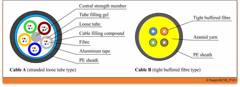
The world of optical communication is intricate, with different cable types designed for specific environments and applications. Today, we’re diving into the structure of two common types of optical fiber cables, as depicted in Figure below, and summarising the findings from an appendix that examined their performance.

Figure

Cable A: The Stranded Loose Tube Outdoor Cable

Cable A represents a quintessential outdoor cable, built to withstand the elements and the rigors of outdoor installation. The cross-section of this cable reveals a complex structure designed for durability and performance:

Central Strength Member: At its core, the cable has a central strength member that provides mechanical stability and ensures the cable can endure the tensions of installation.
Tube Filling Gel: Surrounding the central strength member are buffer tubes secured with a tube filling gel, which protects the fibers from moisture and physical stress.
Loose Tubes: These tubes hold the optical fibers loosely, allowing for expansion and contraction due to temperature changes without stressing the fibers themselves.
Fibers: Each tube houses six fibers, comprising various types specified by the ITU-T, including G.652.D, G.654.E, G.655.D, G.657.A1, G.657.A2, and G.657.B3. This array of fibers ensures compatibility with different transmission standards and conditions.
Aluminium Tape and PE Sheath: The aluminum tape provides a barrier against electromagnetic interference, while the polyethylene (PE) sheath offers physical protection and resistance to environmental factors.

The stranded loose tube design is particularly suited for long-distance outdoor applications, providing a robust solution for optical networks that span vast geographical areas.

Cable B: The Tight Buffered Indoor Cable

Switching our focus to indoor applications, Cable B is engineered for the unique demands of indoor environments:

Tight Buffered Fibers: Unlike Cable A, this indoor cable features four tight buffered fibers, which are more protected from physical damage and easier to handle during installation.
Aramid Yarn: Known for its strength and resistance to heat, aramid yarn is used to reinforce the cable, providing additional protection and tensile strength.
PE Sheath: Similar to Cable A, a PE sheath encloses the structure, offering a layer of defense against indoor environmental factors.

Cable B contains two ITU-T G.652.D fibers and two ITU-T G.657.B3 fibers, allowing for a blend of standard single-mode performance with the high bend-resistance characteristic of G.657.B3 fibers, making it ideal for complex indoor routing.

Conclusion

The intricate designs of optical fiber cables are tailored to their application environments. Cable A is optimized for outdoor use with a structure that guards against environmental challenges and mechanical stresses, while Cable B is designed for indoor use, where flexibility and ease of handling are paramount. By understanding the components and capabilities of these cables, network designers and installers can make informed decisions to ensure reliable and efficient optical communication systems.

Reference

https://www.itu.int/rec/T-REC-G.Sup40-201810-I/en

ITU-T Recommendations for Optical Fibers and Cables

Standards 3 Mins Read

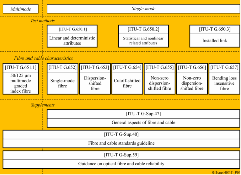
In the realm of telecommunications, the precision and reliability of optical fibers and cables are paramount. The International Telecommunication Union (ITU) plays a crucial role in this by providing a series of recommendations that serve as global standards. The ITU-T G.650.x and G.65x series of recommendations are especially significant for professionals in the field. In this article, we delve into these recommendations and their interrelationships, as illustrated in Figure 1 .

ITU-T G.650.x Series: Definitions and Test Methods

The ITU-T G.650.x series is foundational for understanding single-mode fibers and cables. ITU-T G.650.1 is the cornerstone, offering definitions and test methods for linear and deterministic parameters of single-mode fibers. This includes key measurements like attenuation and chromatic dispersion, which are critical for ensuring fiber performance over long distances.

Moving forward, ITU-T G.650.2 expands on the initial parameters by providing definitions and test methods for statistical and non-linear parameters. These are essential for predicting fiber behavior under varying signal powers and during different transmission phenomena.

For those involved in assessing installed fiber links, ITU-T G.650.3 offers valuable test methods. It’s tailored to the needs of field technicians and engineers who analyze the performance of installed single-mode fiber cable links, ensuring that they meet the necessary standards for data transmission.

ITU-T G.65x Series: Specifications for Fibers and Cables

The ITU-T G.65x series recommendations provide specifications for different types of optical fibers and cables. ITU-T G.651.1 targets the optical access network with specifications for 50/125 µm multimode fiber and cable, which are widely used in local area networks and data centers due to their ability to support high data rates over short distances.

The series then progresses through various single-mode fiber specifications:

ITU-T G.652: The standard single-mode fiber, suitable for a wide range of applications.
ITU-T G.653: Dispersion-shifted fibers optimized for minimizing chromatic dispersion.
ITU-T G.654: Features a cut-off shifted fiber, often used for submarine cable systems.
ITU-T G.655: Non-zero dispersion-shifted fibers, which are ideal for long-haul transmissions.
ITU-T G.656: Fibers designed for a broader range of wavelengths, expanding the capabilities of dense wavelength division multiplexing systems.
ITU-T G.657: Bending loss insensitive fibers, offering robust performance in tight bends and corners.

Historical Context and Current References

It’s noteworthy to mention that the multimode fiber test methods were initially described in ITU-T G.651. However, this recommendation was deleted in 2008, and now the test methods for multimode fibers are referenced in existing IEC documents. Professionals seeking current standards for multimode fiber testing should refer to these IEC documents for the latest guidelines.

Conclusion

The ITU-T recommendations play a critical role in the standardization and performance optimization of optical fibers and cables. By adhering to these standards, industry professionals can ensure compatibility, efficiency, and reliability in fiber optic networks. Whether you are a network designer, a field technician, or an optical fiber manufacturer, understanding these recommendations is crucial for maintaining the high standards expected in today’s telecommunication landscape.

Reference

https://www.itu.int/rec/T-REC-G/e

Power Change during add/remove of channels on filters

Technical 2 Mins Read

Power Change during add/remove of channels on filters

The power change can be quantified as the ratio between the number of channels at the reference point after the channels are added or dropped and the number of channels at that reference point previously. We can consider composite power here and each channel at same optical power in dBm.

So whenever we add or delete number of channels from a MUX/DEMUX/FILTER/WSS following equations define the new changed power.

For the case when channels are added (as illustrated on the right side of Figure 1 ):

where:

A is the number of added channels

U is the number of undisturbed channels

For the case when channels are dropped (as illustrated on the left side of Figure 1):

where:

D is the number of dropped channels

U is the number of undisturbed channels

Figure 1

For example:

– adding 7 channels with one channel undisturbed gives a power change of +9 dB;

– dropping 7 channels with one channel undisturbed gives a power change of –9 dB;

– adding 31 channels with one channel undisturbed gives a power change of +15 dB;

– dropping 31 channels with one channel undisturbed gives a power change of –15 dB;

refer ITU-T G.680 for further study.

HD-FEC & SD-FEC differences

Technical 1 Min Read

Items	HD-FEC	SD-FEC
Definition	Decoding based on hard-bits(the output is quantized only to two levels) is called the “HD(hard-decision) decoding”, where each bit is considered definitely one or zero.	Decoding based on soft-bits(the output is quantized to more than two levels) is called the “SD(soft-decision) decoding”, where not only one or zero decision but also confidence information for the decision are provided.
Application	Generally for non-coherent detection optical systems, e.g., 10 Gbit/s, 40 Gbit/s, also for some coherent detection optical systems with higher OSNR	coherent detection optical systems, e.g., 100 Gbit/s,400 Gbit/s.
Electronics Requirement	ADC(Analogue-to-Digital Converter) is not necessary in the receiver.	ADC is required in the receiver to provide soft information, e.g., coherent detection optical systems.
specification	general FEC per [ITU-T G.975];super FEC per [ITU-T G.975.1].	vendor specific
typical scheme	Concatenated RS/BCH	LDPC(Low density parity check),TPC(Turbo product code)
complexity	medium	high
redundancy ratio	generally 7%	around 20%
NCG	about 5.6 dB for general FEC;>8.0 dB for super FEC.	>10.0 dB
Example(If you asked your friend about traffic jam status on roads and he replies)	maybe fully jammed or free	50-50 but I found othe way free or less traffic

Difference between OTDR and COTDR

Technical 1 Min Read

What is a OTDR ?

Optical Time Domain Reflectometer – also known as an OTDR, is a hardware device used for measurement of the elapsed time and intensity of light reflected on optical fiber.

How it works?

The reflectometer can compute the distance to problems on the fiber such as attenuation and breaks, making it a useful tool in optical network troubleshooting.

The intensity of the return pulses is measured and integrated as a function of time, and is plotted as a function of fiber length.

What is a COTDR?

Coherent Optical Time Domain Reflectometer – also known as a COTDR, An instrument that is used to perform out of service backscattered light measurements on optically amplified line systems.

How it works?

A fiber pair is tested by launching a test signal into the out going fiber and receiving the scattered light on the in-coming fiber. Light scattered in the transmission fiber is coupled to the incoming fiber in the loop-back couplers in each amplifier pair in a repeater.

A walk-through with non linear impairments in optical fiber

Technical 1 Min Read

Non-linear interactions between the signal and the silica fibre transmission medium begin to appear as optical signal powers are increased to achieve longer span lengths at high bit rates. Consequently, non-linear fibre behaviour has emerged as an important consideration both in high capacity systems and in long unregenerated routes. These non-linearities can be generally categorized as either scattering effects (stimulated Brillouin scattering and stimulated Raman scattering) or effects related to the fibre’s intensity dependent index of refraction (self-phase modulation, cross-phase modulation, modulation instability, soliton formation and four-wave mixing). A variety of parameters influence the severity of these non-linear effects, including line code (modulation format), transmission rate, fibre dispersion characteristics, the effective area and non-linear refractive index of the fibre, the number and spacing of channels in multiple channel systems, overall unregenerated system length, as well as signal intensity and source line-width. Since the implementation of transmission systems with higher bit rates than 10 Gbit/s and alternative line codes (modulation formats) than NRZ-ASK or RZ-ASK, described in [b-ITU-T G-Sup.39], non‑linear fibre effects previously not considered can have a significant influence, e.g., intra‑channel cross-phase modulation (IXPM), intra-channel four-wave mixing (IFWM) and non‑linear phase noise (NPN).

Understanding multipliers and divisors value in calculating OTN frame rates (255,239,238,237 etc) for OPUk,ODUk and OTUk

Technical 3 Mins Read

**Multiplicative factor is just a simple math :eg. for ODU1/OPU1=3824/3808={(239*16)/(238*16)}

Here value of multiplication factor will give the number of times for rise in the frame size after adding header/overhead.

Example:let consider y=(x+delta[x])/x; In terms of OTN frame here delta[x] is increment of Overhead.

As we are using Reed Soloman(255,239) i.e we are dividing 4080bytes in sixteen frames (The forward error correction for the OTU-k uses 16-byte interleaved codecs using a Reed- Solomon S(255,239) code. The RS(255,239) code operates on byte symbols.).Hence 4080/16=255.

Try to understand using OTN frames now. I have tried to make it legible.

As we know that OPU1 payload rate= 2.488 Gbps (OC48/STM16) and is frame size is 4*3808 as below.

*After adding OPU1 and ODU1 16 bytes overhead: Frames could be fragmented into following number of chunks.

3808/16 = 238, (3808+16)/16 = 239

So, ODU1 rate: 2.488 x 239/238** ~ 2.499Gbps

*Now after adding FEC bytes

OTU1 rate: ODU1 x 255/239 = 2.488 x 239/238 x 255/239

=2.488 x 255/238 ~2.667Gbps

Now let’s have a small discussion over different multiplier and divisor scenarios that will make it clearer to understand.

We know that an OTU frame 4 * 4080 bytes (= 255 * 16 * 4)

OPU representing the Payload (3824-16) * 4 * 4 = 3808 bytes (= 238 * 16 * 4) .

OPU1 is exactly the rate of STM-16.

Now,

ODU1 = (3824/3808) * OPU1 = ((16 * 239) / (238 16 *)) * OPU1 = (239/238) * STM-16

OTU1 = (4080/3808) * OPU1 = ((255 * 16) / (238 * 16)) * OPU1 = (255/238) * STM-16

OPU2 contains 16 * 4 = 64 bytes of fixed stuff (FS) added to the 1905 to 1920 .

OPU2 * ((238 * 16 * 4-16 * 4) / (238 * 16 * 4)) = STM-64 rate

OPU2 = 238 / (238-1) * STM-64 = 238/237* STM-64 rate

ODU2 = (239/237) * STM-64 rate ,

similarly

OTU2 = ( 255/237) * STM-64 rate

OPU3 Including 2 * 16 * 4 = 128 fixed stuff (FS) bytes added to the 1265 ~ 1280 and 2545 ~ 2560

OPU3 * ((238 * 16 * 4-2 * 16 * 4) / (238 * 16 * 4)) = rate of STM-256

OPU3 = 238 / (238-2) * STM-256 = 238/236 * STM-256

ODU3 = (239 / 236) * STM-256

OTU3 = (255/236) * STM-256

The OTU4 was required to transport ten ODU2e signals, which have a non-SDH based clock frequency as basis. The OTU4 clock should be based on the same SDH clock as the OTU1, OTU2 and OTU3 and not on the 10GBASE-R clock, which determines the ODU2e frequency. An exercise was performed to determine the necessary divider in the factor 255/divider, and the value 227 was found to meet the requirements (factor 255/227). Note that this first analysis has indicated that a future 400 Gbit/s OTU5 could be created using a factor 255/226 and a 1 Tbit/s OTU6 using a factor 255/225.

What is Optical Power Requirement and margin for a optics module’s power?

Interviews 1 Min Read

Optical power tolerance: It refers to the tolerable limit of input optical power, which is the range from sensitivity to overload point.

Optical power requirement: If refers to the requirement on input optical power, realized by adjusting the system (such as adjustable attenuator, fix attenuator, optical amplifier).

Optical power margin: It refers to an acceptable extra range of optical power. For example, “–5/ + 3 dB” requirement is actually a margin requirement.

How to know if errors are due to linear or non-linear issue in an optical link?

Standards 1 Min Read

When the bit error occurs to the system, generally the OSNR at the transmit end is well and the fault is well hidden.

Decrease the optical power at the transmit end at that time. If the number of bit errors decreases at the transmit end, the problem is non-linear problem.

If the number of bit errors increases at the transmit end, the problem is the OSNR degrade problem.

General Causes of Bit Errors

Performance degrade of key boards
Abnormal optical power
Signal-to-noise ratio decrease
Non-linear factor
Dispersion (chromatic dispersion/PMD) factor
Optical reflection
External factors (fiber, fiber jumper, power supply, environment and others)

What are main advantages and drawbacks of EDFAs?

Infographics 1 Min Read

The main advantages and drawbacks of EDFAs are as follows.

Advantages

Commercially available in C band (1,530 to 1,565 nm) and L band (1,560 to 1,605) and up to 84-nm range at the laboratory stage.
Excellent coupling: The amplifier medium is an SM fiber;
Insensitivity to light polarization state;
Low sensitivity to temperature;
High gain: > 30 dB with gain flatness < ±0.8 dB and < ±0.5 dB in C and L band, respectively, in the scientific literature and in the manufacturer documentation
Low noise figure: 4.5 to 6 dB
No distortion at high bit rates;
Simultaneous amplification of wavelength division multiplexed signals;
Immunity to crosstalk among wavelength multiplexed channels (to a large extent)

Drawbacks

Pump laser necessary;
Difficult to integrate with other components;
Need to use a gain equalizer for multistage amplification;
Dropping channels can give rise to errors in surviving channels:dynamic control of amplifiers is necessary.

A short discussion on 980nm and 1480nm pump based EDFA

Technical 4 Mins Read

A short discussion on 980nm and 1480nm pump based EDFA

Introduction

The 980nm pump needs three energy level for radiation while 1480nm pumps can excite the ions directly to the metastable level .

(a) Energy level scheme of ground and first two excited states of Er ions in a silica matrix. The sublevel splitting and the lengths of arrows representing absorption and emission transitions are not drawn to scale. In the case of the 4 I11/2 state, s is the lifetime for nonradiative decay to the I13/2 first excited state and ssp is the spontaneous lifetime of the 4 I13/2 first excited state. (b) Absorption coefficient, a, and emission coefficient, g*, spectra for a typical aluminum co-doped EDF.

The most important feature of the level scheme is that the transition energy between the I15/2 ground state and the I13/2 first excited state corresponds to photon wavelengths (approximately 1530 to 1560 nm) for which the attenuation in silica fibers is lowest. Amplification is achieved by creating an inversion by pumping atoms into the first excited state, typically using either 980 nm or 1480 nm diode lasers. Because of the superior noise figure they provide and their superior wall plug efficiency, most EDFAs are built using 980 nm pump diodes. 1480 nm pump diodes are still often used in L-band EDFAs although here, too, 980 nm pumps are becoming more widely used.

Though pumping with 1480 nm is used and has an optical power conversion efficiency which is higher than that for 980 nm pumping, the latter is preferred because of the following advantages it has over 1480 nm pumping.

It provides a wider separation between the laser wavelength and pump wavelength.
980 nm pumping gives less noise than 1480nm.
Unlike 1480 nm pumping, 980 nm pumping cannot stimulate back transition to the ground state.
980 nm pumping also gives a higher signal gain, the maximum gain coefficient being 11 dB/mW against 6.3 dB/mW for the 1.48
The reason for better performance of 980 nm pumping over the 1.48 m pumping is related to the fact that the former has a narrower absorption spectrum.
The inversion factor almost becomes 1 in case of 980 nm pumping whereas for 1480 nm pumping the best one gets is about 1.6.
Quantum mechanics puts a lower limit of 3 dB to the optical noise figure at high optical gain. 980 nm pimping provides a value of 3.1 dB, close to the quantum limit whereas 1.48 pumping gives a value of 4.2 dB.
1480nm pump needs more electrical power compare to 980nm.

Application

The 980 nm pumps EDFA’s are widely used in terrestrial systems while 1480nm pumps are used as Remote Optically Pumped Amplifiers (ROPA) in subsea links where it is difficult to put amplifiers.For submarine systems, remote pumping can be used in order not to have to electrically feed the amplifiers and remove electronic parts.Nowadays ,this is used in pumping up to 200km.

The erbium-doped fiber can be activated by a pump wavelength of 980 or 1480 nm but only the second one is used in repeaterless systems due to the lower fiber loss at 1.48 mm with respect to the loss at 0.98 mm. This allows the distance between the terminal and the remote amplifier to be increased.

In a typical configuration, the ROPA is comprised of a simple short length of erbium doped fiber in the transmission line placed a few tens of kilometers before a shore terminal or a conventional in-line EDFA. The remote EDF is backward pumped by a 1480 nm laser, from the terminal or in-line EDFA, thus providing signal gain

Vendors

Following are the vendors that manufactures 980nm and 1480nm EDFAs

Basic understanding on Tap ratio for Splitter/Coupler

Technical 2 Mins Read

Basic understanding on Tap ratio for Splitter/Coupler

Fiber splitters/couplers divide optical power from one common port to two or more split ports and combine all optical power from the split ports to one common port (1 × N coupler). They operate across the entire band or bands such as C, L, or O bands. The three port 1 × 2 tap is a splitter commonly used to access a small amount of signal power in a live fiber span for measurement or OSA analysis. Splitters are referred to by their splitting ratio, which is the power output of an individual split port divided by the total power output of all split ports. Popular splitting ratios are shown in Table below; however, others are available. Equation below can be used to estimate the splitter insertion loss for a typical split port. Excess splitter loss adds to the port’s power division loss and is lost signal power due to the splitter properties. It typically varies between 0.1 to 2 dB, refer to manufacturer’s specifications for accurate values. It should be noted that splitter function is symmetrical.

where IL = splitter insertion loss for the split port, dB

Pi = optical output power for single split port, mW

PT = total optical power output for all split ports, mW

SR = splitting ratio for the split port, %

Γe = splitter excess loss (typical range 0.1 to 2 dB), dB

Common splitter applications include

• Permanent installation in a fiber link as a tap with 2%|98% splitting ratio. This provides for access to live fiber signal power and OSA spectrum measurement without affecting fiber traffic. Commonly installed in DWDM amplifier systems.

• Video and CATV networks to distribute signals.

• Passive optical networks (PON).

• Fiber protection systems.

Example with calculation:

If a 0 dBm signal is launched into the common port of a 25% |75% splitter, then the two split ports, output power will be −6.2 and −1.5 dBm. However, if a 0 dBm signal is launched into the 25% split port, then the common port output power will be −6.2 dBm.

Calculation.

Launch power=0 dBm =1mW

Tap is 25%|75%

so equivalent mW power which is linear will be

0.250mW|0.750mW

and after converting them ,dBm value will be

-6.02dBm| -1.24dBm

Some of the common split ratios and their equivalent Optical Power is available below for reference.

What an OTDR can do for you?

Standards 2 Mins Read

The Optical Time Domain Reflectometer (OTDR) is useful for testing the integrity of fiber optic cables. An optical time-domain reflectometer (OTDR) is an optoelectronic instrument used to characterize an optical fiber. An OTDR is the optical equivalent of an electronic time domain reflectometer. It injects a series of optical pulses into the fiber under test. It also extracts, from the same end of the fiber, light that is scattered (Rayleigh backscatter) or reflected back from points along the fiber. The strength of the return pulses is measured and integrated as a function of time, and plotted as a function of fiber length.

Using an OTDR, we can:

1. Measure the distance to a fusion splice, mechanical splice, connector, or significant bend in the fiber.

2. Measure the loss across a fusion splice, mechanical splice, connector, or significant bend in the fiber.

3. Measure the intrinsic loss due to mode-field diameter variations between two pieces of single-mode optical fiber connected by a splice or connector.

4. Determine the relative amount of offset and bending loss at a splice or connector joining two single-mode fibers.

5. Determine the physical offset at a splice or connector joining two pieces of single-mode fiber, when bending loss is insignificant.

6. Measure the optical return loss of discrete components, such as mechanical splices and connectors.

7. Measure the integrated return loss of a complete fiber-optic system.

8. Measure a fiber’s linearity, monitoring for such things as local mode-field pinch-off.

9. Measure the fiber slope, or fiber attenuation (typically expressed in dB/km).

10. Measure the link loss, or end-to-end loss of the fiber network.

11. Measure the relative numerical apertures of two fibers.

12. Make rudimentary measurements of a fiber’s chromatic dispersion.

13. Measure polarization mode dispersion.

14. Estimate the impact of reflections on transmitters and receivers in a fiber-optic system.

15. Provide active monitoring on live fiber-optic systems.

16. Compare previously installed waveforms to current traces.

Factors That Contribute to Chromatic Dispersion and how to Combat it?

Technical 2 Mins Read

Chromatic dispersion affects all optical transmissions to some degree.These effects become more pronounced as the transmission rate increases and fiber length increases.

Factors contributing to increasing chromatic dispersion signal distortion include the following:

1. Laser spectral width, modulation method, and frequency chirp. Lasers with wider spectral widths and chirp have shorter dispersion limits. It is important to refer to manufacturer specifications to determine the total amount of dispersion that can be tolerated by the lightwave equipment.

2. The wavelength of the optical signal. Chromatic dispersion varies with wavelength in a fiber. In a standard non-dispersion shifted fiber (NDSF G.652), chromatic dispersion is near or at zero at 1310 nm. It increases positively with increasing wavelength and increases negatively for wavelengths less than 1310 nm.

3. The optical bit rate of the transmission laser. The higher the fiber bit rate, the greater the signal distortion effect.
4. The chromatic dispersion characteristics of fiber used in the link. Different types of fiber have different dispersion characteristics.
5. The total fiber link length, since the effect is cumulative along the length of the fiber.
6. Any other devices in the link that can change the link’s total chromatic dispersion including chromatic dispersion compensation modules.
7. Temperature changes of the fiber or fiber cable can cause small changes to chromatic dispersion. Refer to the manufacturer’s fiber cable specifications for values.

Methods to Combat Link Chromatic Dispersion

1. Change the equipment laser with a laser that has a specified longer dispersion limit. This is typically a laser with a more narrow spectral width or a laser that has some form of precompensation. As laser spectral width decreases, chromatic dispersion limit increases.
2. For new construction, deploy NZ-DSF instead of SSMF fiber.NZ-DSF has a lower chromatic dispersion specification.
3. Insert chromatic dispersion compensation modules (DCM) into the fiber link to compensate for the excessive dispersion. The optical loss of the DCM must be added to the link optical loss budget and optical amplifiers may be required to compensate.
4. Deploy a 3R optical repeater (re-amplify, reshape, and retime the signal) once a link reaches chromatic dispersion equipment limit.
5. For long haul undersea fiber deployment, splicing in alternating lengths of dispersion compensating fiber can be considered.
6. To reduce chromatic dispersion variance due to temperature, buried cable is preferred over exposed aerial cable.

MapYourTech

Industry Relevant Contents and Advanced Tools for Optical Engineering Professionals

Fiber optic technology

Definition and Physical Meaning

Quantum Limit and Physical Interpretation

Factors Affecting Noise Figure

Gain and Population Inversion

Input Power Dependence

Wavelength Dependence

Temperature Effects

EDFA Specifications

Temperature Sensitivity

Cascaded Amplifiers and Noise Accumulation

Friis' Formula and Cascaded Amplifier Systems

Key Insights from Friis' Formula

OSNR Evolution in Multi-span Systems

Practical Example: OSNR Calculation in a Multi-span System

Multi-Stage Amplifier Design

EDFA Models and Cascaded Performance

Automatic Laser Shutdown (ALS) and Safety

Network Applications and Optimization Strategies for Optical Amplifiers

Network Segment Requirements

Access Networks

Metro/Regional Networks

Long-haul Networks

Economic Implications of Noise Figure

Operational Optimization Strategies

1. Gain Optimization

2. Tilt Management

3. Temperature Control

4. Fiber Plant Optimization

Noise Figure Design Guidelines

Future Trends in Noise Figure Technology

EDFA Implementation Examples

Metro Network Design

Regional Network Design

Specialized Applications

Conclusion

Introduction to 400G ZR

Key features of 400G ZR include:

Emergence of 400G ZR+

Key enhancements in 400G ZR+ include:

ZR vs. ZR+: A Comparative Analysis

The Future Outlook

Reference

Classification of OA Devices

Applications and Configurations

Characteristics of Optical Amplifiers

Optically Amplified Transmitters and Receivers

Understanding Through Practical Examples

Advanced Applications of Optical Amplifiers

Technological Innovations and Challenges

Future of Optical Amplifiers in Industry

References

The Challenge of ASE Noise

Understanding OSNR

Reference System for OSNR Estimation

Estimating OSNR in a Cascaded System

Simplifying the Equation

Practical Implications for Network Design

Conclusion

References

Cable A: The Stranded Loose Tube Outdoor Cable

Cable B: The Tight Buffered Indoor Cable

Conclusion

Reference

ITU-T G.650.x Series: Definitions and Test Methods

ITU-T G.65x Series: Specifications for Fibers and Cables

Historical Context and Current References

Conclusion

Reference

Power Change during add/remove of channels on filters

A short discussion on 980nm and 1480nm pump based EDFA

Introduction

Application

Vendors

Basic understanding on Tap ratio for Splitter/Coupler