Generic selectors
Exact matches only
Search in title
Search in content
Post Type Selectors
Articles
lp_course
lp_lesson
Back
Courses
Optical Network Fundamentals
Network Architecture & Design
Advanced Technologies
Network Operations & Management
Fiber Optics & Components
DWDM Technology
Transport Networks & OTN
Testing & Performance
Protection & Reliability
Network Automation
Articles
Optical Networking Fundamentals
Network Planning & Design
Networking Automation
Network Analysis
Network Testing
Network Management
Networking Standards
Network Security
Technology Article
Optical Trends & News
Tools
Design & Planning
OptiMap Pro: Professional Optical Network Designer and Planner
Simulators
OSNR vs GOSNR Professional Simulator
MapYourHCF Splice Loss Simulator
Optical link OSNR Simulator
MapYourOTDR Simulator and Viewer
Optical Networks Fiber Cut & Availability Simulator
Optical C+L SRS Visualiser
EDFA Gain and NF Simulator
Calculators
Optical Channels Composite Power Calculator
Optical Link Attenuation Calculator
Optical General Utility
Optical Spectral Efficiency Calculator
Optical Signal Reach Calculator
Optical Fiber Latency Calculator
Shannon Limit Calculator
Developer Tools
MapYourHTML
MapYourDiff+
MapYourMarkdown Editor
MapYourFile Comparison
Resources
Optical Networking Troubleshooting Guide
Optical Network Alarms Knowledge Base
Optical Network Specifications Reference
Infographics Collection
Optical Networking Technologies Collection (80+)
Optical Fibers Infographics
WDM Infographics
OTN Infographics
SDH/SONET/PDH Infographics
Optical Impairments Infographics
Ethernet Infographics
OTN Standards & ITU-T Standard Explorer
Optical Glossary
Career
Market Research & Analytics for Optical Industry
Interview Insights
Salary Insights
Optical Networking Interview Preparation Quick Refresher
Books
MapYourTech eBooks
Optical Network Communications: An Engineer’s Perspective
Automation for Network Engineers Using Python and Jinja2
Interview Buddy Series
Account
Log In
Profile
Pricing
Home
Posts tagged “noise figure”
noise figure
Showing 1 - 6 of 6 results
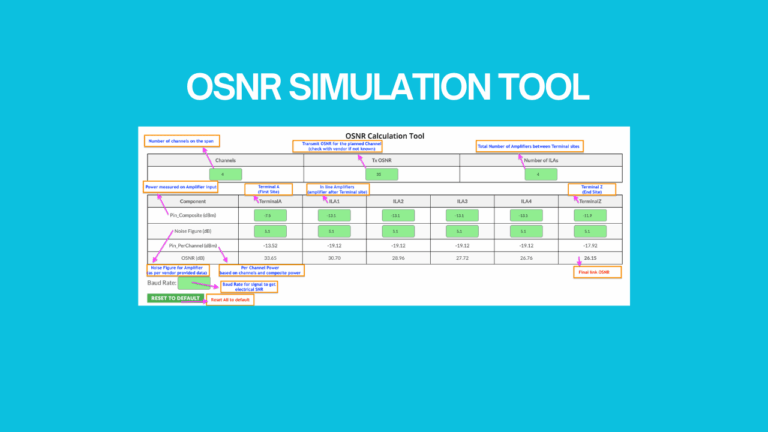
Understanding the OSNR Simulation Tool
Based on my experience ,I have seen that Optical Engineers need to estimate Optical Signal-to-Noise Ratio (OSNR) often specially when...
Free
March 26, 2025
Read more
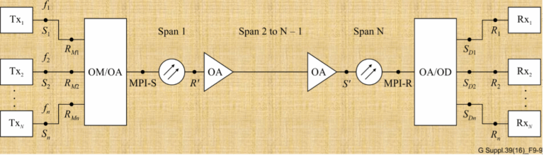
Noise Concatenation in Optical Amplifier Chains
Optical networks are the backbone of the internet, carrying vast amounts of data over great distances at the speed of...
Free
March 26, 2025
Read more
Understanding Noise Figure in Amplifiers: Definition, Importance, and How to Reduce It
When working with amplifiers, grasping the concept of noise figure is essential. This article aims to elucidate noise figure, its...
Free
March 26, 2025
Read more
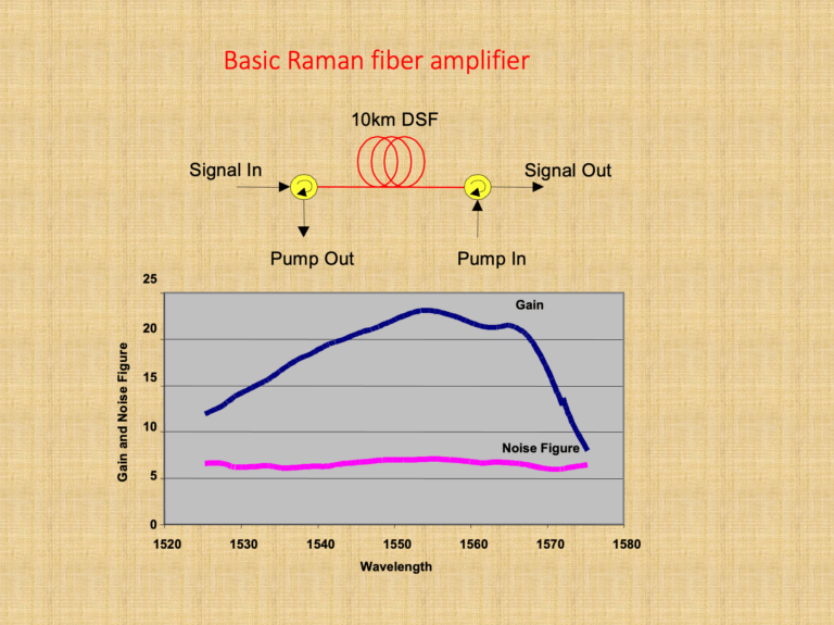
Raman Amplifier and Negative noise figure analysis
In the context of Raman amplifiers, the noise figure is typically not negative. However, when comparing Raman amplifiers to other...
Free
March 26, 2025
Read more
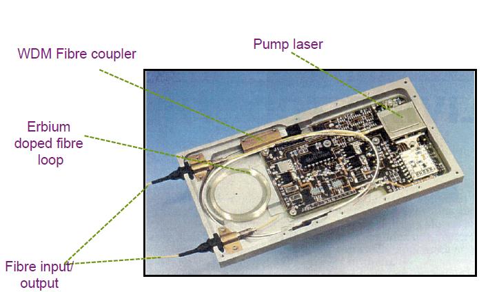
What are main advantages and drawbacks of EDFAs?
The main advantages and drawbacks of EDFAs are as follows. Advantages Commercially available in C band (1,530 to 1,565 nm)...
Free
March 26, 2025
Read more
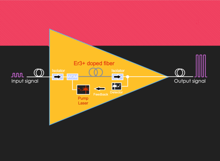
A short discussion on 980nm and 1480nm pump based Erbium Doped Fiber Amplifiers (EDFA)
The 980nm pump needs three energy level for radiation while 1480nm pumps can excite the ions directly to the metastable...
Free
March 26, 2025
Read more
Explore
Articles
Analysis
Automation
Free
Fundamentals
Management
Planning & Design
Premium
Security
Standards
Technical
Testing
Trends & News
Filter
Articles
Free
Premium
Reset
Explore Courses
Tags
automation
ber
Chromatic Dispersion
coherent optical transmission
Data transmission
DWDM
edfa
EDFAs
Erbium-Doped Fiber Amplifiers
fec
Fiber optics
Fiber optic technology
Forward Error Correction
Latency
modulation
network automation
network management
Network performance
noise figure
optical
optical amplifiers
optical automation
Optical communication
Optical fiber
Optical network
optical network automation
optical networking
Optical networks
Optical performance
Optical signal-to-noise ratio
Optical transport network
OSNR
OTN
Q-factor
Raman Amplifier
SDH
Signal integrity
Signal quality
Slider
submarine
submarine cable systems
submarine communication
submarine optical networking
Telecommunications
Ticker
Follow us
Children Education
Idiom Meaning
Shayari.net
Course Title
Course description and key highlights
Course Content
Course Details
Enroll in Course