MapYourBasics Series
Raman Amplifier and Negative Noise Figure Analysis
The figure looks impossible: a noise figure below 0 dB seems to claim an amplifier that improves signal-to-noise ratio. It does not. The negative number is an accounting choice that compares distributed gain against the lumped-amplifier reference engineers grew up with. Here is what the number means, when it turns negative, and where the physics stops it.
1. Introduction
If you have spent any time reading Raman amplifier datasheets or system design notes, you have probably come across a noise figure quoted as a negative number, and it likely stopped you for a moment. A negative noise figure looks impossible, because noise figure is defined as the ratio of the signal-to-noise ratio at the input to the signal-to-noise ratio at the output, and any real amplifier adds some spontaneous-emission noise of its own, which can only degrade that ratio. By that definition the value in decibels should always come out positive, and for a single amplifier considered on its own, it does.
The negative number you see quoted for a distributed Raman amplifier is therefore measuring something different. It is not the intrinsic noise figure of the device in isolation, but what is called the effective or equivalent noise figure, and the difference between those two quantities is the whole point. The intrinsic noise figure answers the question "how much noise does this amplifier add." The equivalent noise figure answers a more practical question that system engineers actually care about: "what discrete amplifier, placed at the end of this span of fiber, would give me the same signal-to-noise ratio at the receiver that this distributed amplifier delivers." When you spread Raman gain along the transmission fiber rather than lumping it at one point, the answer to that second question can fall below 0 dB, and the negative sign turns out to carry real, useful meaning about reach rather than signalling any violation of physics.
It is worth being precise about one framing error that comes up often, because the original explanations of this effect tend to soften it. The negative value is not simply "the difference between two amplifiers" written as a single number. A distributed Raman amplifier genuinely has a negative equivalent noise figure in its own right, defined against a discrete-amplifier reference, and the sections that follow build that result up from the physics step by step. If you want the gain mechanism itself before going further, the MapYourTech explainer on how a Raman amplifier works covers the stimulated-scattering process this article assumes.
2. What Noise Figure Actually Measures
Before the negative figure makes sense, it helps to be clear about what noise figure is actually measuring, because the two amplifier types arrive at their noise through quite different routes. In both cases noise figure captures the signal-to-noise penalty a device imposes between its input and output, but the physical origin of that penalty is what separates an EDFA from a Raman stage. In an erbium-doped fiber amplifier the dominant noise source is amplified spontaneous emission. Erbium ions raised to their excited state do not all wait to be stimulated by the signal; some decay spontaneously and emit photons in random directions, and once those photons are travelling along the fiber the amplifier cannot tell them apart from the signal, so it amplifies them too. The amount of this ASE scales with the gain and with how completely the erbium is inverted, which is why a fully inverted EDFA has a theoretical noise figure floor of 3 dB and why practical units land somewhere between 4 and 6 dB once you account for input coupling loss and incomplete inversion. That same noise accumulates span after span, an effect explored in the MapYourTech treatment of why every span adds ASE.
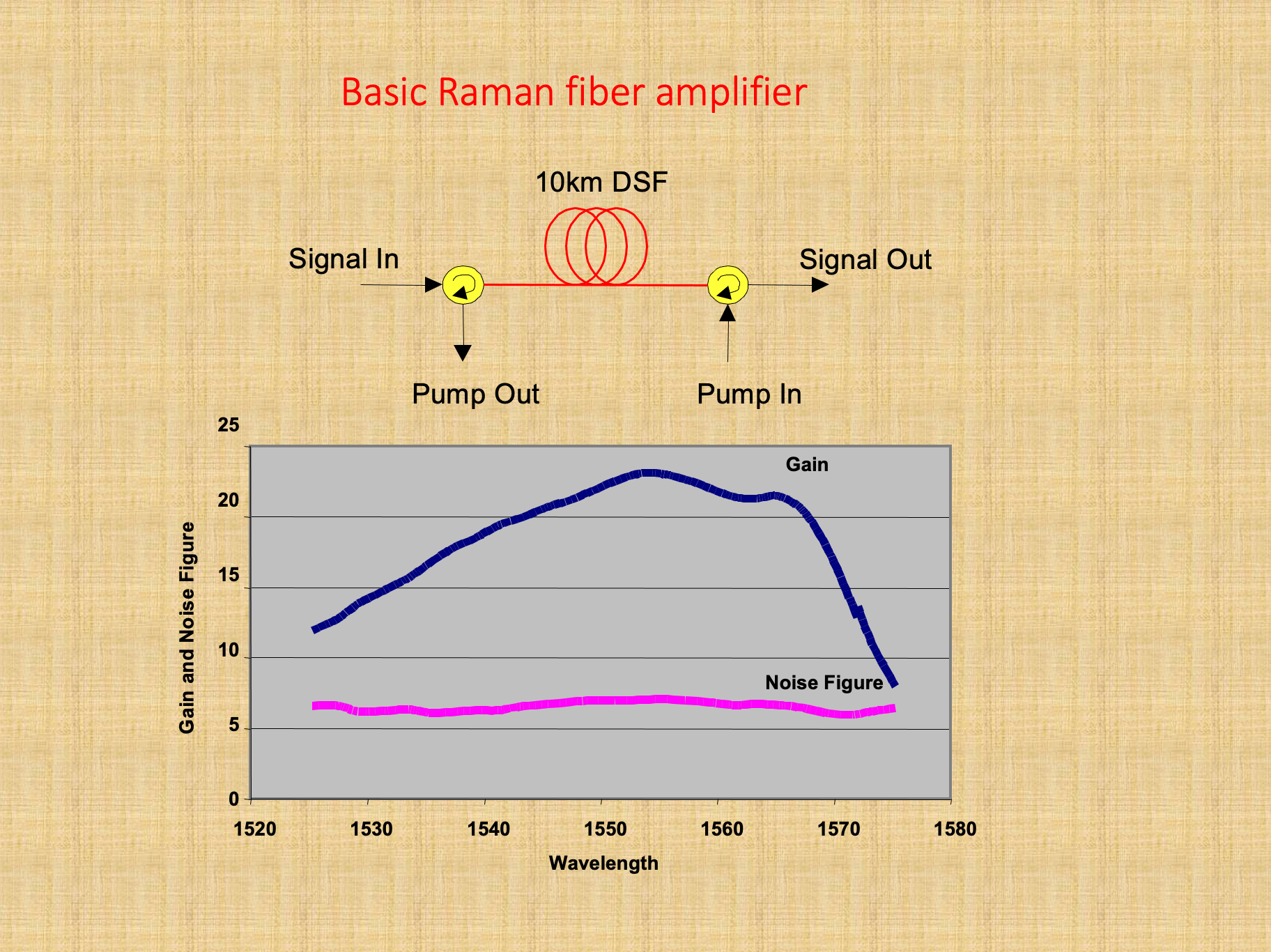
A Raman amplifier generates its noise differently, even though the end result is a comparable noise figure. Here a high-power pump near 1450 nm interacts with the molecular vibrations of the silica itself, handing energy to the signal through stimulated Raman scattering. Just as with the EDFA, not every interaction is the useful one: some pump photons scatter spontaneously rather than into the signal, producing broadband noise photons that the pump then amplifies along with everything else. So the noise floor of a Raman stage is set by spontaneous Raman scattering rather than by erbium ASE, and for a discrete Raman amplifier considered on its own it works out to roughly the same 4 to 6 dB you would expect from an EDFA. The interesting behaviour appears only when the gain is distributed.
Intrinsic noise figure for any single amplifier, Raman or EDFA, is positive in dB. The sub-zero number only appears for the equivalent noise figure of a distributed amplifier, where the gain medium is the transmission fiber itself.
3. The Equivalent Noise Figure Definition
The cleanest way to define the equivalent noise figure is operationally, in terms of an experiment you could imagine running. Picture the distributed Raman amplifier delivering some signal-to-noise ratio at the receiver. Now ask what single discrete amplifier, dropped in at the end of the same span of fiber, you would have to use to land on that exact same receiver signal-to-noise ratio. The noise figure of that hypothetical discrete amplifier is the equivalent noise figure of the distributed one. This is the reference frame system engineers reach for almost without thinking, because for decades the mental model of an amplified link has been a passive span of fiber followed by a lumped gain block, not gain smeared continuously along the glass.
That reference frame is exactly why the number can come out negative, and the reason is worth sitting with for a moment. A lumped amplifier waiting at the end of a span only goes to work after the signal has already lost most of its power crawling through tens of kilometres of fiber, so by the time it amplifies, it is boosting a weak signal sitting close to the accumulated noise, and it lifts signal and noise together. Distributed Raman gain does its work earlier, topping the signal up while it is still travelling and before it has decayed to its lowest point, which keeps the signal riding higher above the noise floor across the whole span. When you then compare the two against the same receiver target, the distributed approach simply needs less help at the end, and that deficit is what the negative sign records. The way the signal power actually evolves along the fiber is the physical picture behind all of this, and the geometry of where the gain concentrates is taken further in the MapYourTech note on the clean-fiber zone in Raman links.
Equivalent (effective) noise figure of a distributed Raman amplifier — ITU-T G-series form
NFeff = NFLA + 10 · log10( PASE,Raman / (GRaman · hν · νr) + 1 )
Where NFLA is the noise figure of the discrete line amplifier, GRaman is the on-off (linear) gain of the distributed Raman stage, PASE,Raman is the ASE power the Raman stage produces, hν is photon energy, and νr is the reference bandwidth. As Raman on-off gain rises, the bracketed term shrinks and NFeff falls — eventually below 0 dB.
There is a second, more intuitive way to write the same thing, and it is the form that makes the negative sign obvious. The effective noise figure of a distributed stage comes out as its intrinsic noise figure minus the span loss that its distributed gain has already offset ahead of the reference plane. As long as the amount of loss the gain compensates stays smaller than the intrinsic noise figure, the result is positive; the moment the compensated loss grows larger than the intrinsic noise figure, the result tips below zero. Section 5 works this through with real numbers, but the principle is simple enough to state in one line: the distributed stage is not manufacturing signal-to-noise ratio out of nothing, it is sidestepping the loss penalty that a lumped amplifier has no choice but to pay before it can amplify.
4. The Gain Threshold for a Negative Result
How much distributed gain you need before the number actually turns negative is governed by the on-off Raman gain, which is just the ratio of the output signal power with the pump switched on to the output power with the pump off. Published modelling and laboratory measurements put the crossover at around 10 dB of on-off gain. Below that point the equivalent noise figure stays stubbornly positive, because the distributed gain has not yet offset enough loss to overcome the intrinsic noise figure. Push past it and the number slides below zero, and it keeps falling as you add more on-off gain. The improvement does not run away forever, though, and Section 6 explains where it stops.
Which end of the span you pump from matters just as much as how hard you pump, and in deployed systems backward pumping is the configuration that delivers the benefit cleanly. With backward, or counter-propagating, pumping the pump light is launched at the receive end and travels against the signal, so the Raman gain piles up near the far end of the span, which is precisely where the signal has grown weakest and needs the help most. There is a second advantage that is easy to overlook: because the pump and the signal are moving in opposite directions, any fluctuation in the pump power gets averaged out over the transit rather than imprinting itself on the signal, so the transfer of pump relative intensity noise stays low. Forward, or co-propagating, pumping has its own appeal, giving more gain for each watt of pump because it acts where the signal is still strong, but it pays for that efficiency by coupling pump intensity noise straight onto the signal, which is why it is used carefully and often only in combination with backward pumping.
5. Computing the Effective Noise Figure
With the principle in place, it is worth actually putting numbers through it, because seeing the negative figure emerge from a calculation makes it far more convincing than any amount of explanation. The loss-offset form is the natural starting point. A distributed Raman stage spread over a length of transmission fiber presents an effective noise figure equal to its intrinsic noise figure minus the span loss its distributed gain has already made up. The comparison, as always, is against a discrete amplifier sitting at the end of that same fiber, and that reference amplifier has to swallow the full span loss before it ever amplifies, so its noise contribution gets referred back through all of that attenuation. The distributed stage never pays that toll, and the formula simply books the difference.
Effective noise figure, loss-offset form
NFeff ≈ NFint − Lcomp
NFint is the intrinsic noise figure of the Raman stage (dB); Lcomp is the span loss the distributed gain offsets ahead of the reference point (dB). When the compensated loss exceeds the intrinsic noise figure, NFeff goes below 0 dB. The number reports loss the reference amplifier would have incurred and the distributed stage did not.
Take a representative span and let the values be realistic ones. A backward-pumped distributed Raman stage working over the final stretch of standard single-mode fiber will typically carry an intrinsic noise figure somewhere around 5.5 dB, a figure set by the spontaneous Raman scattering and by the loss of coupling the pump in at the receive end. Suppose the distributed gain offsets on the order of 9 dB of fiber loss ahead of the reference plane, which is a perfectly ordinary amount for a counter-propagating pump. Substituting these straight into the loss-offset form gives the result below.
Representative span — distributed Raman pre-amplifier
NFeff ≈ 5.5 − 9.0 = −3.5 dB
A discrete amplifier cannot reach this figure. Its floor is the 3 dB quantum limit, and any real unit sits above it. The distributed stage reports −3.5 dB because the comparison is against a lumped amplifier that would have amplified a signal already 9 dB weaker.
It is worth being blunt about what that −3.5 dB is and is not, because this is exactly where the older explanations tend to go soft. It is not a small positive noise figure with the sign flipped for effect, and it is not merely the gap between two amplifiers written as one number. It is a direct statement that this distributed architecture hands the receiver a better signal-to-noise ratio than any discrete amplifier could ever manage at the same span loss, because the discrete amplifier is stuck paying a fiber-attenuation penalty before it amplifies and the distributed stage simply is not. The negative sign is that avoided penalty, made visible.
The more common real-world arrangement pairs the distributed Raman stage with a discrete line amplifier sitting behind it, so it is worth running that case too. Take a line-amplifier noise figure NFLA of 6.5 dB and a distributed Raman on-off gain GRaman of 9.3 dB, and feed them into the combined-stage expression. The stage effective noise figure works out to roughly 1 dB, which is already comfortably below the 3 dB floor a discrete amplifier can never beat, and the Raman contribution on its own is running negative before the line amplifier adds its share on top.
What this buys you is reach, and the size of the effect is striking. Held against a fixed receiver OSNR target — the kind of budget worked through in the MapYourTech walkthrough of OSNR calculation for an amplified cascaded span — this design reaches a theoretical limit of around 19 spans with no forward error correction at all, and once you add standard soft-decision FEC the same line stretches well beyond 40 spans. None of that extra margin came from turning up the launch power or reworking the channel plan; it came entirely from moving where the gain happens.
The reason it works comes back to the same picture from the start: the Raman stage delivers its gain before the signal has decayed across the full 80 km, so the line amplifier behind it is handed a stronger signal to work with and ends up referring proportionally less of its own ASE into the final signal-to-noise ratio.
| Property | Discrete EDFA | Distributed Raman |
|---|---|---|
| Gain location | Lumped, at span end | Spread along transmission fiber |
| Dominant noise source | Amplified spontaneous emission | Spontaneous Raman scattering |
| Intrinsic noise figure | 4–6 dB (3 dB floor) | 4–6 dB |
| Effective noise figure | Equals intrinsic | Below 0 dB achievable |
| Signal amplified when | After full-span decay | Before significant decay |
| Pump power | Tens of mW | Above 1 W |
6. The Rayleigh-Backscatter Floor
At this point a reasonable instinct is to keep cranking up the Raman gain and watch the effective noise figure dive ever more negative, but the physics does not cooperate, and the reason it stops is worth understanding because it shapes how these systems are actually built. The limit comes from double Rayleigh backscattering. Glass is never perfectly uniform, and a tiny fraction of the signal light is always scattering backward off the frozen-in density fluctuations of the fiber. Most of that backscattered light simply heads back toward the transmitter and is lost, but a second scattering event can turn some of it around again so that it rejoins the forward-travelling signal, now delayed and out of step with the original. To the receiver this re-scattered light looks like a faint, smeared copy of the signal, a multipath-interference noise that the distributed gain unhelpfully amplifies right along with everything else.
The trouble is that this re-scattered noise grows faster than the noise-figure benefit once the on-off gain climbs past about 20 dB, so beyond that point you are adding more interference than improvement. Published analysis puts the lowest achievable equivalent noise figure somewhere around 33 dB of on-off gain, and past that the double Rayleigh contribution takes over completely and the number starts climbing back up. This is why real distributed Raman systems do not chase the deepest possible negative figure. They settle for a moderate on-off gain where the benefit is real but the backscatter is still under control, and more often than not they pair the Raman stage with a discrete amplifier rather than asking the distributed gain to do everything on its own.
Pushing the on-off gain higher in the hope of driving the equivalent noise figure further negative eventually works against you. Once you are past roughly 20 dB of on-off gain, double Rayleigh backscattering brings in multipath interference that no amount of extra pump power can scrub out. The sensible operating window is therefore a moderate gain, and quite often a bidirectional pumping scheme that balances the forward pump's RIN transfer against the backward pump's signal-to-noise advantage.
7. Why Hybrid Raman-EDFA Spans Use It
All of this is why long-haul and submarine systems so often put a distributed Raman pre-amplifier in front of a discrete EDFA rather than choosing one or the other. The pairing is a deliberate way to capture the equivalent-noise-figure benefit while staying well short of the Rayleigh floor that would punish an all-Raman design. The Raman stage does its job first, lifting the signal-to-noise ratio at the point where the EDFA picks it up, and because the EDFA is now working on a healthier signal it injects less ASE of its own for the same end-of-span power. Published hybrid designs report the combined noise figure coming out around 3 dB better than an equivalent EDFA-only span, which translates into close to 2 dB of additional nonlinear OSNR margin.
It would be tempting to assume that 2 dB of OSNR converts directly into a matching jump in capacity, but the relationship is not nearly that generous, and it is worth understanding why. The same low channel powers that keep the nonlinear penalties in check also limit how freely that extra margin can be spent, and nonlinear effects such as four-wave mixing and stimulated Brillouin scattering quietly cap what the system can actually carry. One published hybrid design, for instance, saw only about a 9.5 percent capacity increase despite the clear noise-figure improvement. This OSNR-against-reach balancing act is the same one that governs every amplified line, and it is taken further in the MapYourTech overview of what and why of the Raman amplifier, with the configuration specifics laid out in the short note on distributed Raman amplification.
There is one more reason distributed Raman keeps its place in the toolkit, and it has nothing to do with noise figure at all. It is the only practical way to put gain in parts of the spectrum where erbium simply does not work. Since the gain comes from the fiber's own Raman response rather than from a doped section of glass, you get to choose where the gain sits just by choosing the pump wavelength, anywhere from roughly 1300 to 1600 nm. That band flexibility is one of the headline points among the advantages of using a Raman amplifier, and if you want the numbers side by side, the MapYourTech questions on Raman amplifiers reference runs through pump wavelengths, gain bandwidth, and the typical gain figures you can expect.
Takeaway: A distributed Raman amplifier's equivalent noise figure can fall below 0 dB because it is measured against a lumped amplifier that would have amplified a fully decayed signal. The negative sign reports avoided loss, not created signal-to-noise ratio. The benefit appears above roughly 10 dB on-off gain, reaches its best value near 33 dB, and is capped beyond about 20 dB by double Rayleigh backscattering — which is why deployed systems run moderate Raman gain, usually as a pre-amplifier ahead of an EDFA.
8. Conclusion
The negative noise figure, then, is real, well defined, and genuinely useful, as long as you keep straight which noise figure anyone is talking about. The intrinsic noise figure of any single amplifier stays firmly above 0 dB, because spontaneous emission guarantees it. The equivalent noise figure is a different and more practical quantity, measuring a distributed Raman stage against the discrete amplifier you would otherwise have used, and because the distributed gain keeps the signal high all along the span instead of rescuing it at the very end, that comparison lands below 0 dB once the gain passes its threshold. Nothing in this picture breaks the second law; it simply rewards a smarter placement of gain.
For anyone designing a line the takeaway is refreshingly concrete. A negative equivalent noise figure on a Raman stage is telling you there is reach margin available that no lumped amplifier could give you at the same span loss, and you are free to spend it on longer spans, more spans, or a higher modulation order. The only discipline the physics asks of you is to respect the Rayleigh-backscatter floor, hold the on-off gain to a moderate level, and lean on an EDFA alongside the Raman stage rather than pushing distributed gain past the point where it starts to hurt.
References
- ITU-T, Handbook on Optical Fibres, Cables and Systems — Optical Systems Design and Distributed Raman Amplification, International Telecommunication Union.
- ITU-T Recommendation G.665, Generic characteristics of Raman amplifiers and Raman amplified subsystems, ITU-T Study Group 15.
- R. Ramaswami, K. N. Sivarajan and G. H. Sasaki, Optical Networks: A Practical Perspective — Optical Amplifiers, Morgan Kaufmann.
- J. Bromage, "Raman Amplification for Fiber Communications Systems," Journal of Lightwave Technology.
Sanjay Yadav, "Optical Network Communications: An Engineer's Perspective" — Bridge the Gap Between Theory and Practice in Optical Networking.
Developed by MapYourTech Team
For educational purposes in Optical Networking Communications Technologies
Note: This guide is based on industry standards, best practices, and real-world implementation experiences. Specific implementations may vary based on equipment vendors, network topology, and regulatory requirements. Always consult with qualified network engineers and follow vendor documentation for actual deployments.
Feedback Welcome: If you have any suggestions, corrections, or improvements to propose, please feel free to write to us at [email protected]

Optical Communications & Network Automation Expert | Author of 3 Books for Optical Engineers | Founder, MapYourTech
Optical networking engineer with nearly two decades of experience across DWDM, OTN, coherent optics, submarine systems, and cloud infrastructure. Founder of MapYourTech. Read full bio →
Follow on LinkedInRelated Articles on MapYourTech


Continue Reading This Article
Sign in with a free account to unlock the full article and access the complete MapYourTech knowledge base.