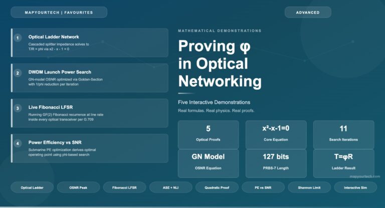
Golden Ratio Proofs in Optical Networking Optical Engineering Proving φ in Optical Networking: Five Demonstrations Real formulas. Real physics. Real...
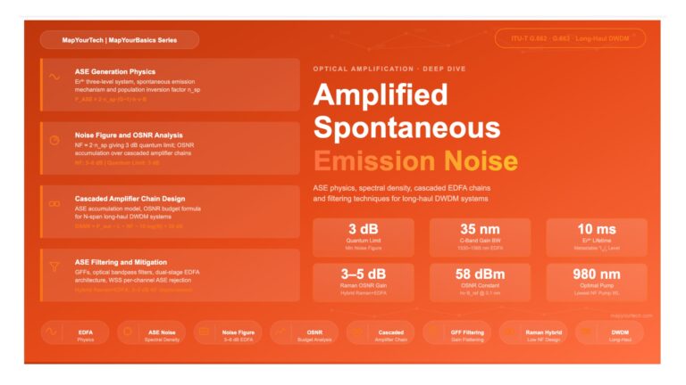
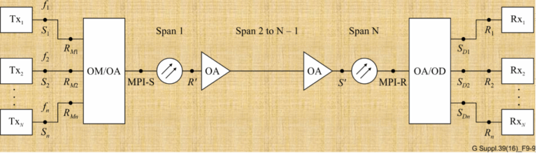
Amplified Spontaneous Emission (ASE) Noise in EDFA Systems Amplified Spontaneous Emission (ASE) Noise in EDFA Systems A comprehensive engineering reference...
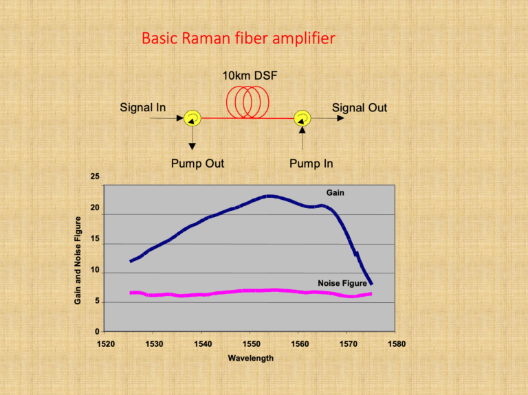
Raman Amplifier and Negative Noise Figure Analysis MapYourBasics Series Raman Amplifier and Negative Noise Figure Analysis The figure looks impossible:...
Get new articles, courses & exclusive offers first
Follow MapYourTech on LinkedIn for exclusive updates — new technical articles, course launches, member discounts, tool releases, and industry insights straight to your feed.