
Basic understanding on Tap ratio for Splitter and Coupler
Understanding Power Division, Insertion Loss, and Practical Applications in Modern Optical Networks
1. Introduction to Fiber Optic Splitters and Couplers
Fiber optic splitters and couplers are fundamental passive components in modern optical communication networks. These devices enable the distribution of optical signals from a single input to multiple outputs (splitting) or the combination of multiple optical signals into a single output (coupling). Unlike active components that require external power, splitters operate purely through the physics of light propagation, making them highly reliable and maintenance-free.
The importance of fiber optic splitters in telecommunications infrastructure cannot be overstated. They serve as the backbone of passive optical networks (PONs), CATV distribution systems, and dense wavelength division multiplexing (DWDM) networks. Understanding the principles of tap ratios, splitting ratios, and insertion loss is essential for network engineers, system designers, and anyone involved in optical network planning and deployment.
Why Splitters Matter
In fiber-to-the-home (FTTH) deployments, a single fiber from the central office can serve dozens of customers through strategically placed splitters. In DWDM systems, small tap couplers allow engineers to monitor live traffic without disrupting service. The versatility and reliability of optical splitters make them indispensable in modern network architectures.
The Role of Splitters in Optical Networks
Fiber splitters serve multiple critical functions in optical communication systems:
- Signal Distribution: Distributing optical power from one source to multiple destinations, enabling point-to-multipoint communication architectures.
- Network Monitoring: Providing tap points for optical spectrum analyzers (OSAs) and power meters without interrupting live traffic.
- Protection Switching: Enabling redundant path configurations in fiber protection schemes for enhanced network reliability.
- Cost Optimization: Reducing infrastructure costs by allowing a single optical line terminal (OLT) to serve multiple optical network units (ONUs).
Operating Characteristics
Fiber optic splitters and couplers operate across entire wavelength bands without wavelength-selective filtering. Common operating bands include:
- O-band (Original): 1260-1360 nm - Used primarily in PON upstream transmission
- E-band (Extended): 1360-1460 nm - Extended wavelength range for additional capacity
- S-band (Short): 1460-1530 nm - Short wavelength band
- C-band (Conventional): 1530-1565 nm - Most common for DWDM and long-haul transmission
- L-band (Long): 1565-1625 nm - Long wavelength band for extended DWDM capacity
The broadband nature of fiber splitters makes them wavelength-agnostic, meaning they divide power proportionally across all wavelengths present in the input signal. This characteristic is crucial for wavelength division multiplexed (WDM) systems where multiple wavelengths coexist on the same fiber.
2. Fundamental Principles of Optical Power Division
The Physics of Optical Splitting
Optical power division in fiber splitters relies on controlled coupling of light between optical waveguides. When two or more optical fibers or waveguides are brought into close proximity, an evanescent field extends beyond the core boundary, allowing energy transfer between the guides through a phenomenon known as directional coupling.
The splitting mechanism can be implemented through two primary technologies:
Fused Biconical Taper (FBT) Technology
In FBT splitters, two or more optical fibers are twisted together and then fused and tapered under heat. The tapering process brings the fiber cores into proximity, enabling evanescent wave coupling. The degree of tapering controls the coupling ratio, allowing precise control over the split ratio. FBT splitters are known for their low cost, low insertion loss, and excellent reliability.
Planar Lightwave Circuit (PLC) Technology
PLC splitters use photolithography and semiconductor fabrication techniques to create waveguides on a glass substrate. The waveguide pattern defines the splitting structure, typically using a cascade of Y-branches or multimode interference (MMI) regions. PLC splitters excel in applications requiring high split counts (1×32, 1×64, or higher) with uniform splitting ratios and excellent wavelength uniformity.
Symmetry and Bidirectional Operation
Critical Concept: Splitter Reciprocity
It is essential to note that splitter function is symmetrical. This means a splitter can operate equally well in both directions. A device that splits light from one input to multiple outputs can also combine light from multiple inputs to a single output with the same power distribution ratios. This reciprocity is fundamental to understanding splitter behavior in bidirectional applications such as PON systems.
For example, if a 25%|75% splitter directs 25% of input power to Port A and 75% to Port B when light enters the common port, then when light enters Port A, 25% reaches the common port, with the remaining power distributed according to the coupling mechanism. This symmetry allows the same component to function as both a splitter and a combiner.
3. Understanding Tap Ratio and Splitting Ratio
Definition and Terminology
The splitting ratio (SR) defines how optical power is distributed among the output ports of a splitter. It is expressed as the percentage of total output power delivered to each split port. For a 1×N splitter (one input, N outputs), the splitting ratios of all outputs sum to 100%, neglecting excess loss.
Splitting Ratio Formula:
Where: SR = splitting ratio for port i (%)
Pi = optical output power for individual split port i (mW)
PT = total optical power output for all split ports (mW)
A tap ratio typically refers to a specific type of splitter where a small percentage of power is "tapped off" for monitoring or measurement, while the majority passes through to the primary output. The nomenclature uses the format "X%|Y%" where X represents the tap port percentage and Y represents the through port percentage.
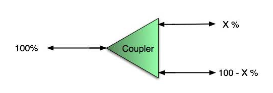
Figure 1: Optical coupler showing tap ratio concept with X% and (100-X)% power distribution
Common Splitting Ratios
Optical splitters are manufactured in standard splitting ratios to meet various application requirements. Here are the most common configurations:
Equal Split Ratios (Balanced Splitters)
- 50/50 (1×2): Divides power equally between two outputs - used in interferometers and balanced detection systems
- 33.3/33.3/33.3 (1×3): Three-way equal split for triple-redundant monitoring
- 25/25/25/25 (1×4): Four-way equal split for quad distribution
Unequal Split Ratios (Asymmetric Splitters)
- 1/99: Minimal tap for ultra-low-intrusion monitoring in high-power systems
- 2/98: Low-intrusion tap, commonly installed in DWDM amplifier spans
- 5/95: Standard monitoring tap with minimal signal degradation
- 10/90: Balanced monitoring tap for OSA analysis
- 20/80: Higher tap ratio for detailed spectrum analysis
- 30/70: Moderate split for dual-path systems
High Split Count Configurations
- 1×8: Eight-way split, common in small PON deployments
- 1×16: Sixteen-way split, standard for medium PON systems
- 1×32: Thirty-two-way split, most common in GPON/EPON networks
- 1×64: Sixty-four-way split, used in next-generation PON (NG-PON2)
- 1×128: Ultra-high split count for massive subscriber density
Important Consideration
Custom splitting ratios can be manufactured for specialized applications, but standard ratios are more cost-effective and readily available. When specifying splitters, always consider the total link budget and whether the insertion loss will impact system performance margins.
4. Insertion Loss Calculation and Analysis
Components of Insertion Loss
The total insertion loss of a fiber optic splitter consists of two main components:
- Theoretical Splitting Loss: The inherent loss due to power division, calculated from the splitting ratio
- Excess Loss: Additional loss due to material absorption, scattering, imperfect coupling, and manufacturing tolerances
Insertion Loss Formula:
Where: IL = insertion loss for the split port (dB)
SR = splitting ratio for the split port (%)
Γe = excess loss (typically 0.1 to 2 dB)
Understanding Excess Loss
Excess loss (Γe) represents the difference between the actual insertion loss and the theoretical minimum loss based on the splitting ratio. This additional loss arises from:
- Material Absorption: Light absorption in the fiber or waveguide material
- Fresnel Reflections: Reflections at interfaces between different refractive indices
- Mode Field Mismatch: Imperfect matching between input and output mode field diameters
- Manufacturing Imperfections: Waveguide roughness, dimensional variations, and alignment errors
- Splice Losses: Losses at the connection points between the splitter and fiber pigtails
Typical Excess Loss Values
FBT Splitters: 0.1 to 0.3 dB for low split counts (1×2 to 1×4), increasing to 0.5-1.0 dB for higher splits
PLC Splitters: 0.8 to 1.5 dB for standard products, with premium devices achieving 0.5-0.8 dB
Custom Splitters: May exhibit higher excess loss (1.5-2.5 dB) depending on specifications
Uniformity and Balance
In addition to insertion loss, splitter uniformity is critical for equal-split configurations. Uniformity specifies the maximum variation in insertion loss between any two output ports. For example, a 1×32 splitter might specify ±0.8 dB uniformity, meaning all 32 outputs have insertion losses within a 1.6 dB range of each other.
Poor uniformity can lead to:
- Unequal received power levels at different subscriber locations in PON networks
- Difficulty in maintaining system margins across all branches
- Reduced overall network capacity due to weakest-link limitations
- Increased complexity in network planning and power budgeting
5. Types and Configurations of Fiber Splitters
Classification by Port Configuration
1×N Splitters (Star Configuration)
The most common type, featuring one input port and N output ports. Power from the input is divided among all outputs according to the specified splitting ratio. Configurations range from 1×2 to 1×128, with 1×32 being the standard for PON deployments.
2×N Splitters (Dual Input)
Two input ports can be used independently or combined to feed N output ports. These devices enable protection switching where two redundant sources can be combined, or they can function as two independent 1×N splitters in a single package.
M×N Splitters (Matrix Configuration)
Multiple inputs and outputs allowing complex routing configurations. While less common, these specialized devices serve in applications requiring flexible signal distribution and combining in the same component.
Classification by Physical Package
Bare Fiber Splitters
Minimal packaging with 250 μm coated fibers directly exiting the device. These compact splitters are ideal for space-constrained installations and integration into larger assemblies. They require careful handling due to exposed fibers.
Steel Tube Packaged Splitters
The splitter element is housed in a small stainless steel tube (typically 1-3 mm diameter, 40-60 mm length) with 900 μm buffered fiber pigtails. This provides mechanical protection while maintaining a small form factor, suitable for cabinet and rack mounting.
ABS Box Splitters
Larger plastic enclosures (typically 100×80×10 mm) containing the splitter with strain relief and cable management. Connectorized versions include SC, LC, or FC/APC connectors for plug-and-play installation. These are standard in outdoor cabinets and distribution boxes.
Rack Mount Modules
19-inch rack-mountable modules containing multiple splitters with front-panel connectors. These modular systems allow centralized splitter management in data centers and central office environments, with typical 1U height housing 16 to 64 splitter ports.
Specialized Configurations
Polarization-Maintaining (PM) Splitters
Designed to preserve the polarization state of light through the splitting process. These specialized devices use PM fiber and alignment techniques to maintain polarization extinction ratios exceeding 20 dB, essential for coherent communication systems and quantum key distribution.
Wavelength-Flattened Splitters
Optimized for minimal insertion loss variation across wide wavelength ranges. Standard splitters may exhibit 0.5-1.0 dB variation from 1260 to 1625 nm, while wavelength-flattened versions reduce this to <0.3 dB, critical for wideband WDM applications.
High-Power Splitters
Engineered to handle elevated optical power levels (>1 W per port) without damage or performance degradation. These devices use larger core fibers, enhanced heat dissipation, and specialized coatings to support high-power fiber laser and amplifier applications.
6. Common Applications in Network Infrastructure
Passive Optical Networks (PON)
PON systems represent the most widespread application of fiber optic splitters. In GPON (Gigabit-capable Passive Optical Network), EPON (Ethernet Passive Optical Network), and next-generation PON systems, splitters enable point-to-multipoint architecture where a single OLT port at the central office serves multiple ONUs at customer premises.
PON Architecture Example
Scenario: FTTH deployment serving a residential area
Configuration: 1×32 splitter placed in a street cabinet
Result: One fiber from CO splits to 32 homes, dramatically reducing fiber count and infrastructure costs
The downstream signal at 1490 nm (data) and 1550 nm (video) broadcasts to all ONUs, with MAC-layer filtering ensuring each customer receives only their traffic. Upstream transmission at 1310 nm uses TDMA to prevent collisions, with the OLT coordinating transmission time slots for each ONU.
DWDM System Monitoring
In DWDM networks, small-tap-ratio splitters (typically 1/99 or 2/98) are permanently installed in fiber spans to provide access points for optical spectrum analysis, power monitoring, and performance verification. This enables network operators to:
- Monitor channel power levels across the DWDM grid
- Detect and analyze optical signal-to-noise ratio (OSNR)
- Verify wavelength accuracy and stability
- Troubleshoot transmission impairments without service interruption
- Perform continuous performance monitoring for proactive maintenance
Standard Practice
The 2/98 tap ratio has become an industry standard for DWDM monitoring because it introduces minimal penalty (approximately 0.1 dB) to the through path while providing sufficient power for accurate OSA measurements. These taps are typically installed immediately after amplifier outputs and at strategic mid-span locations.
CATV and Video Distribution
Cable television and video distribution networks extensively use optical splitters to deliver broadcast content from headends to multiple subscribers. The analog nature of RF-over-fiber transmission in CATV systems places stringent requirements on splitter linearity and uniformity.
Typical CATV splitter deployments involve:
- Primary distribution from headend using 1×4 or 1×8 splitters
- Secondary distribution with 1×8 or 1×16 splitters at fiber nodes
- Final distribution to homes via coaxial cable from fiber nodes
- Cascade limits of 2-3 splitter stages to maintain signal quality
Fiber Protection Systems
Network redundancy and protection schemes employ splitters/combiners to implement diverse routing and automatic protection switching:
- 1+1 Protection: Signal splits to primary and backup paths; receiver selects best signal
- 1:1 Protection: Splitter enables monitoring of backup path while primary carries traffic
- 1:N Protection: One backup path protects N working paths using splitter/switch combinations
Fiber Sensor Networks
Distributed fiber optic sensing systems use splitters to interrogate multiple sensor elements:
- Fiber Bragg grating (FBG) sensor arrays for structural monitoring
- Distributed temperature sensing (DTS) in oil and gas pipelines
- Acoustic sensing for perimeter security and seismic monitoring
- Vibration detection in railway and highway infrastructure
Test and Measurement
Laboratory and field test equipment incorporates splitters for:
- Simultaneous connection of multiple test instruments to a single fiber
- Reference arm implementation in coherent test systems
- Power splitting for comparison measurements
- Signal distribution in automated test setups
7. Practical Calculation Examples
Example 1: Basic Power Splitting Calculation
Scenario: 25%|75% Splitter with 0 dBm Input
Given Information:
• Input power: 0 dBm = 1 mW
• Splitter configuration: 25%|75%
• Assumed excess loss: 0.2 dB
Step 1: Calculate Linear Power Distribution
Total input power: 1 mW
Port A (25%): 0.25 mW
Port B (75%): 0.75 mW
Step 2: Convert to dBm
Port A: 10 × log₁₀(0.25) = -6.02 dBm
Port B: 10 × log₁₀(0.75) = -1.24 dBm
Step 3: Add Excess Loss
Port A: -6.02 - 0.2 = -6.22 dBm
Port B: -1.24 - 0.2 = -1.44 dBm
Result: With 0 dBm input, the 25% port outputs approximately -6.2 dBm and the 75% port outputs approximately -1.5 dBm (accounting for excess loss).
Key Insight: Reciprocity
Due to splitter symmetry, if we launch 0 dBm into the 25% port (Port A), the common port will output -6.2 dBm. The coupling ratio determines bidirectional behavior, not the direction of light propagation.
Example 2: PON Link Budget Analysis
Scenario: GPON System with 1×32 Splitter
System Parameters:
• OLT transmit power: +2 dBm
• Fiber attenuation: 0.35 dB/km
• Total fiber distance: 20 km
• Splitter: 1×32 (equal split)
• ONU receiver sensitivity: -28 dBm
• System margin requirement: 3 dB
Step 1: Calculate Fiber Loss
Fiber loss = 0.35 dB/km × 20 km = 7.0 dB
Step 2: Calculate Splitter Insertion Loss
Theoretical splitting loss = 10 × log₁₀(32) = 15.05 dB
Excess loss (assumed): 1.0 dB
Total splitter loss = 15.05 + 1.0 = 16.05 dB
Step 3: Calculate Additional Losses
Connector losses (4 connectors @ 0.3 dB): 1.2 dB
Splice losses (2 splices @ 0.1 dB): 0.2 dB
Step 4: Calculate Received Power
Received power = +2 dBm - 7.0 - 16.05 - 1.2 - 0.2 = -22.45 dBm
Step 5: Verify Link Budget
Available margin = -22.45 - (-28) = 5.55 dB
Required margin = 3 dB
Result: System meets requirements with 2.55 dB excess margin
Example 3: DWDM Tap Monitoring
Scenario: OSA Monitoring with 2/98 Tap
System Configuration:
• DWDM signal level: +5 dBm (per channel)
• Number of channels: 80
• Tap ratio: 2/98
• OSA dynamic range: -60 dBm
• Required OSNR measurement accuracy: ±0.5 dB
Step 1: Calculate Tap Port Power
Theoretical tap loss = 10 × log₁₀(0.02) = -16.99 dB
Adding 0.1 dB excess loss = -17.09 dB
Tap port power per channel = +5 - 17.09 = -12.09 dBm
Step 2: Calculate Through Port Loss
Theoretical through loss = 10 × log₁₀(0.98) = -0.088 dB
Adding 0.1 dB excess loss = -0.188 dB
Through port power = +5 - 0.188 = +4.81 dBm per channel
Step 3: Verify OSA Measurement Capability
Signal at tap port: -12.09 dBm
OSA sensitivity: -60 dBm
Measurement margin: -12.09 - (-60) = 47.91 dB
Result: Excellent signal level for accurate OSNR measurements
Step 4: Impact on Main Signal Path
Power reduction: 0.188 dB (negligible impact on link budget)
Conclusion: 2/98 tap provides optimal balance between monitoring capability and signal path impact
Interactive Splitter Calculator
Use this interactive calculator to analyze splitter configurations from 1×2 to 1×9. Choose equal or custom splitting ratios and get complete power distribution analysis with insertion loss calculations.
Configuration
8. Comprehensive Splitting Ratio Reference Tables
1×2 Splitter Configurations
| Type | Split Ratio (%) | Typical Insertion Loss (dB) Port 1 | Port 2 |
Linear Power (mW) for 1 mW Input |
|---|---|---|---|
| 1×2 | 50|50 | 3.2|3.2 | 0.500|0.500 |
| 1×2 | 45|55 | 3.7|2.8 | 0.450|0.550 |
| 1×2 | 40|60 | 4.2|2.4 | 0.400|0.600 |
| 1×2 | 35|65 | 4.8|2.1 | 0.350|0.650 |
| 1×2 | 30|70 | 5.4|1.8 | 0.300|0.700 |
| 1×2 | 25|75 | 6.2|1.5 | 0.250|0.750 |
| 1×2 | 20|80 | 7.2|1.2 | 0.200|0.800 |
| 1×2 | 15|85 | 8.4|0.91 | 0.150|0.850 |
| 1×2 | 10|90 | 10|0.66 | 0.100|0.900 |
| 1×2 | 5|95 | 13|0.42 | 0.050|0.950 |
| 1×2 | 2|98 | 17|0.29 | 0.020|0.980 |
| 1×2 | 1|99 | 20|0.24 | 0.010|0.990 |
1×3 and 1×4 Splitter Configurations
| Type | Split Ratio (%) | Insertion Loss (dB) | Application |
|---|---|---|---|
| 1×3 | 10|45|45 | 10|3.7|3.7 | Monitoring with dual distribution |
| 1×3 | 20|40|40 | 7.2|4.2|4.2 | Balanced monitoring |
| 1×3 | 30|35|35 | 5.4|4.8|4.8 | Three-way distribution |
| 1×3 | 33.3|33.3|33.3 | 4.9|4.9|4.9 | Equal three-way split |
| 1×3 | 40|30|30 | 4.2|5.4|5.4 | Primary with dual backup |
| 1×3 | 50|25|25 | 3.2|6.2|6.2 | Half power with dual tap |
| 1×3 | 60|20|20 | 2.4|7.2|7.2 | Dominant path with monitoring |
| 1×3 | 70|15|15 | 1.8|8.4|8.4 | Through with dual monitoring |
| 1×3 | 80|10|10 | 1.2|10|10 | Low-intrusion dual tap |
| 1×4 | 25|25|25|25 | 6.2|6.2|6.2|6.2 | Equal four-way distribution |
High Split Count Configurations (PON Applications)
| Configuration | Theoretical Loss (dB) | Typical Total Loss (dB) | Max Distance @ 0.35 dB/km | Typical Application |
|---|---|---|---|---|
| 1×4 | 6.0 | 6.8 - 7.5 | 60+ km | Small PON, CATV primary distribution |
| 1×8 | 9.0 | 10.0 - 10.8 | 50 km | Medium PON, branch distribution |
| 1×16 | 12.0 | 13.0 - 14.0 | 40 km | Standard PON, MDU applications |
| 1×32 | 15.0 | 16.5 - 17.5 | 30 km | GPON/EPON standard deployment |
| 1×64 | 18.1 | 19.5 - 21.0 | 20 km | NG-PON2, ultra-high density |
| 1×128 | 21.1 | 23.0 - 25.0 | 10 km | Future PON, massive MDU |
Note on Table Values
All insertion loss values include typical excess loss of 0.2 dB for 1×2 configurations and 0.8-1.5 dB for higher split counts. Actual values vary by manufacturer and technology (FBT vs PLC). Always consult manufacturer datasheets for specific product specifications. The "Max Distance" assumes a 28 dB link budget (typical for Class B+ PON) after accounting for splitter loss and 2 dB margin.
9. Best Practices and Implementation Guidelines
Network Design Considerations
Link Budget Planning
- Always calculate total link budget including all splitters, connectors, splices, and fiber attenuation
- Include adequate system margin (minimum 3 dB) to account for aging, temperature variations, and future degradation
- Consider worst-case scenarios with maximum fiber distance and highest-loss splitter output port
- Account for bidirectional asymmetry in PON systems where upstream (1310 nm) has higher fiber loss than downstream (1490/1550 nm)
Splitter Placement Strategy
- Centralized Splitting: Single splitter location near OLT - simpler management but requires more fiber distribution
- Distributed Splitting: Cascade of smaller splitters - reduces initial fiber deployment but increases maintenance points
- Hybrid Approach: Combination of centralized and distributed - balances flexibility and cost for mixed density areas
Cascading Limitations
Avoid excessive splitter cascading. Each additional splitter stage adds insertion loss and potentially degrades uniformity. Best practice limits cascades to 2-3 stages maximum. For example, a 1×4 followed by four 1×8 splitters (creating 1×32 effective split) is acceptable, but further cascading would compromise link budget.
Installation Best Practices
Environmental Protection
- Use properly rated enclosures for outdoor installations - minimum IP65 for aerial/buried applications
- Ensure adequate ventilation to prevent condensation in sealed enclosures
- Protect splitter pigtails from excessive bending (minimum 30 mm bend radius for standard fiber)
- Secure fiber coils properly to prevent stress on splitter connections
- Use gel-filled enclosures in direct-buried applications for moisture protection
Connector Management
- Always clean connectors before mating - use proper cleaning procedures with approved solvents and tools
- Inspect connectors with microscope before connection to verify end-face cleanliness
- Use dust caps on all unused ports to prevent contamination
- Label all fibers clearly for easy identification and troubleshooting
- Maintain service loops for future modifications and repairs
Testing and Verification
Acceptance Testing
Upon installation, perform comprehensive testing to verify splitter performance:
- Insertion Loss Measurement: Verify each output port meets specifications using calibrated optical power meter
- Return Loss Testing: Ensure return loss >50 dB to prevent reflections that degrade system performance
- Uniformity Verification: For equal-split configurations, confirm all outputs are within specified uniformity range
- Visual Inspection: Check for proper strain relief, adequate bend radius, and secure mounting
Troubleshooting Common Issues
High Insertion Loss
Possible Causes:
- Contaminated or damaged connectors - clean or replace
- Excessive fiber bending near splitter - relieve strain and maintain proper bend radius
- Defective splitter - replace with known-good unit
- Wrong wavelength measurement - verify test equipment wavelength matches application
Poor Uniformity
Possible Causes:
- Temperature variations across splitter - ensure stable environment
- Polarization-dependent loss (PDL) effects - use polarization-insensitive splitters for high-performance applications
- Manufacturing defects - verify splitter meets specifications or replace
Documentation and Maintenance
- Maintain accurate as-built documentation including splitter locations, ratios, and serial numbers
- Document insertion loss measurements at installation for future comparison
- Update network management systems with splitter configuration and capacity
- Schedule periodic inspections and testing per organizational maintenance procedures
- Track splitter performance trends to identify degradation before service impact
Safety Considerations
Laser Safety Warning
Never look directly into fiber ends or splitter ports, even when you believe no light is present. Optical power at 1310, 1490, and 1550 nm wavelengths is invisible to the human eye but can cause permanent retinal damage. Always use proper optical power meters to verify fiber status before handling. Follow all laser safety regulations and use appropriate personal protective equipment.
10. Conclusion and Key Takeaways
Fiber optic splitters and couplers represent essential building blocks of modern optical communication infrastructure. Their ability to passively divide and combine optical signals without external power makes them invaluable for applications ranging from residential broadband access to enterprise DWDM networks. Understanding the principles of tap ratios, splitting ratios, and insertion loss is fundamental to successful network design and deployment.
Essential Concepts to Remember
- Splitting Ratio Defines Power Distribution: The percentage of output power delivered to each port determines the insertion loss and application suitability
- Insertion Loss = Theoretical + Excess: Total loss includes both the fundamental splitting loss and additional manufacturing/coupling losses
- Splitters Are Bidirectional: The symmetry of splitter operation allows the same device to function as both divider and combiner
- Link Budget Is Critical: Always account for all loss sources including splitters, fiber, connectors, and splices with adequate system margin
- Choose Appropriate Technology: FBT for low split counts and cost optimization, PLC for high splits and uniformity requirements
Summary of Common Configurations
- 1%|99% to 5%|95%: Ultra-low-intrusion monitoring in high-value transmission systems
- 10%|90% to 20%|80%: Standard monitoring taps for DWDM and test applications
- 25%|75% to 40%|60%: Asymmetric distribution for protection switching and unbalanced loads
- 50%|50%: Balanced distribution for dual-path systems and interferometry
- 1×8 to 1×32: Standard PON configurations serving residential and business customers
- 1×64 and beyond: Next-generation PON and ultra-high-density deployments
Future Trends and Developments
As optical networks continue to evolve, splitter technology advances to meet emerging requirements:
- Higher Split Counts: 1×128 and 1×256 splitters enabling more efficient PON deployments
- Wavelength-Selective Splitting: Integration of WDM filters with splitters for sophisticated signal routing
- Low-Loss PLC Technology: Continued reduction in excess loss improving system reach
- Integrated Assemblies: Complete plug-and-play modules combining splitters, connectors, and management hardware
- Harsh Environment Solutions: Ruggedized splitters for industrial, military, and aerospace applications
The fundamental principles covered in this guide provide the foundation for understanding and implementing fiber optic splitters effectively. Whether designing a new PON deployment, adding monitoring capability to an existing DWDM network, or planning a CATV distribution system, proper attention to splitting ratios, insertion loss budgets, and best practices ensures optimal network performance and reliability.
Educational Note: This comprehensive guide is based on industry standards, manufacturer specifications, and real-world implementation experiences in optical networking. Specific implementations may vary based on equipment vendors, network topology, regulatory requirements, and environmental conditions. Always consult with qualified network engineers, follow manufacturer documentation, and adhere to relevant safety standards for actual deployments. The information provided is for educational purposes and should serve as a foundation for further study and professional development in fiber optic communications.
Unlock Premium Content
Join over 400K+ optical network professionals worldwide. Access premium courses, advanced engineering tools, and exclusive industry insights.
Already have an account? Log in here