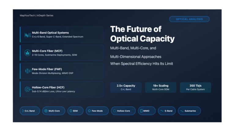
The Future of Optical Capacity: Multi-Band, Multi-Core, and Multi-Dimensional Approaches – Part 1 The Future of Optical Capacity: Multi-Band, Multi-Core,...
Multi-Vendor ROADM Interoperability – Part 1: Introduction & Architecture Multi-Vendor ROADM Interoperability in Optical Transport Networks Introduction The optical networking...
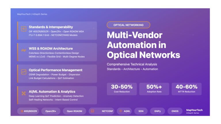
Multi-Vendor Integration in Optical Networks: A Comprehensive Technical Analysis Multi-Vendor Automation in Optical Networks: A Comprehensive Technical Analysis Introduction The...
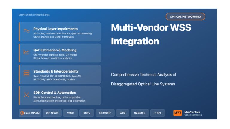
Multi-Vendor WSS Integration in Optical Line Systems: Comprehensive Technical Guide Multi-Vendor WSS Integration in Optical Line Systems Comprehensive Technical Guide:...
Multi-Vendor WSS Integration in Optical Line Systems: Comprehensive Technical Analysis Multi-Vendor WSS Integration in Optical Line Systems Comprehensive Technical Analysis...