
Digital Twin vs Simulator: The Distinction That Matters for Optical Planning
What makes a model a true digital twin versus a simulation tool — and why the difference shapes how operators plan, optimize, and operate modern optical networks.
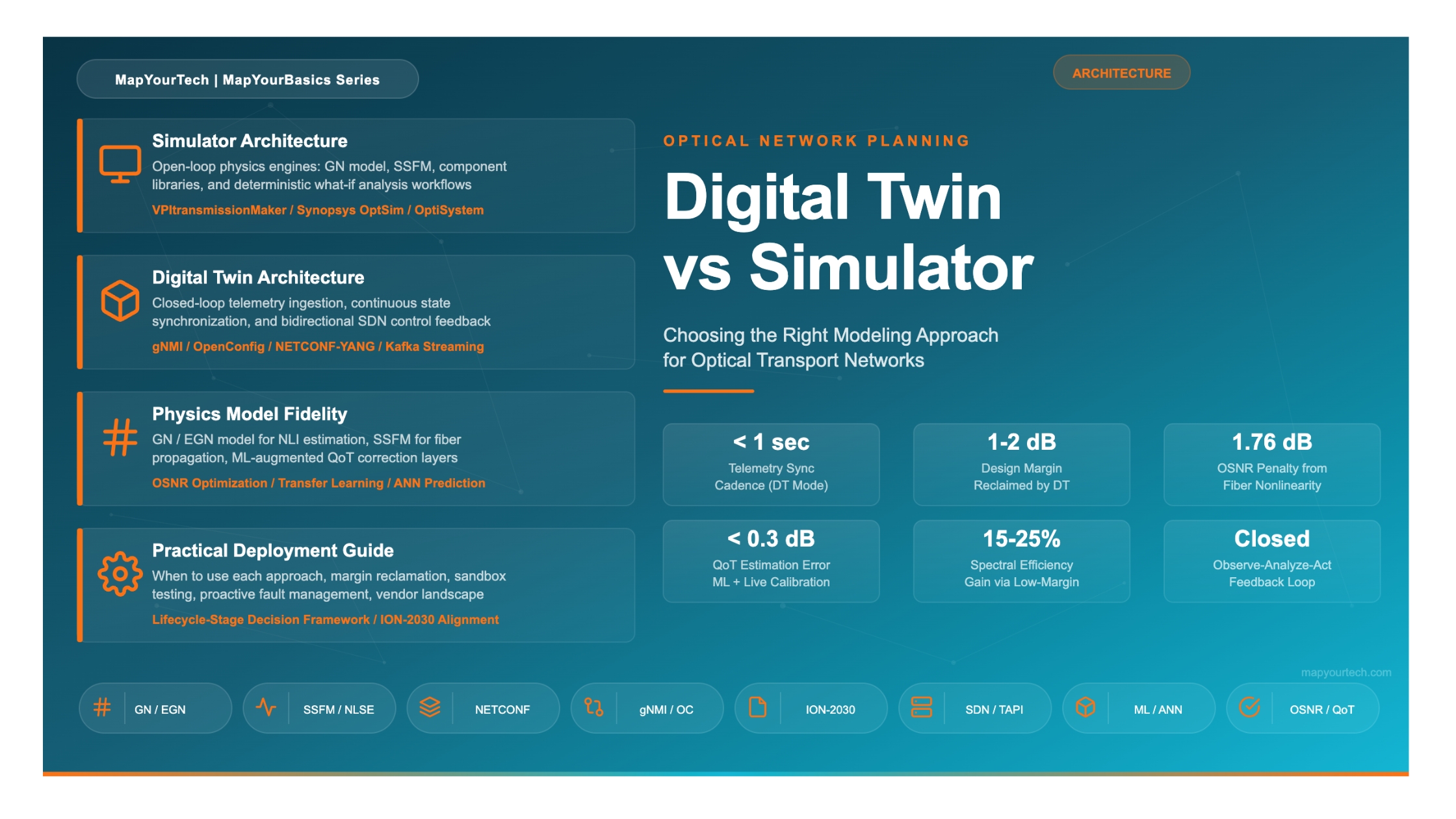
At a Glance
1. Introduction
For decades, optical network planners have relied on simulation software to model fiber propagation, estimate Optical Signal-to-Noise Ratio (OSNR), and evaluate link budgets before committing capital to new routes. Tools such as VPItransmissionMaker, Synopsys OptSim, and Optiwave OptiSystem have allowed engineers to test designs against physics-based models of chromatic dispersion, nonlinear interference, and amplifier noise — all in a controlled, offline environment.
More recently, the term digital twin has entered the optical networking vocabulary, driven by advances in streaming telemetry, machine learning, and Software-Defined Networking (SDN). Industry bodies including ITU-T Study Group 15, the IOWN Global Forum, and the Optical Internetworking Forum (OIF) have positioned network digital twins as a path toward autonomous, self-optimizing optical transport. The ITU-T ION-2030 framework, formally launched in 2025 and advanced at OFC 2026, explicitly names digital twins as a core enabling technology for intelligent optical networks.
Yet the two terms — simulator and digital twin — are often used interchangeably, creating confusion for planners, architects, and operations teams. This article draws a clear technical boundary between them, explains the physics they share, identifies the capabilities that separate them, and provides a practical framework for selecting the right approach based on the task at hand.
2. Fundamentals: What Defines Each Approach
2.1 Optical Network Simulator
An optical network simulator is a software environment that models the physical behavior of optical components and transmission systems using deterministic or statistical algorithms. The engineer provides a set of input parameters — fiber type, span lengths, amplifier placement, channel plan, modulation format — and the simulator produces predicted outputs such as OSNR, Bit Error Rate (BER), Q-factor, or signal constellation quality.
Simulators operate in an open-loop fashion. They have no connection to a live network, receive no real-time data, and cannot push configuration changes back to physical equipment. Their value lies in answering "what if" questions: What happens if we add a span? What is the maximum reach for 64QAM at this baud rate? How much OSNR margin does a new ROADM node consume? These questions are answered by running the physics model forward under user-defined conditions.
Established simulation platforms in the optical domain include VPItransmissionMaker Optical Systems for system-level propagation modeling, Synopsys OptSim for link-level design, and vendor-specific network planning tools that embed the Gaussian Noise (GN) model or Split-Step Fourier Method (SSFM) for fiber propagation calculations.
2.2 Optical Network Digital Twin
A digital twin is a continuously synchronized, software-based replica of a live optical network. It ingests real-time telemetry — OSNR values, power levels, BER readings, amplifier gain profiles, transponder DSP metrics — and uses that data to maintain an up-to-the-moment model of the physical layer. Where a simulator starts from a clean design, a digital twin starts from the network as it exists right now, with all its accumulated aging, splice degradation, filter narrowing, and environmental drift.
The defining characteristic is the bidirectional feedback loop. A digital twin does not just observe the network; it can propose and, in some architectures, execute changes. When a Quality of Transmission (QoT) estimation indicates that a lightpath will soon breach its BER threshold, the digital twin can trigger a proactive reroute, adjust launched power, or recommend a modulation format change — actions that flow from the virtual model back into the physical network through SDN controllers or NETCONF/YANG interfaces.
ITU-T SG15 has discussed the role of digital twins in intelligent transport networks extensively, framing the digital twin as a technology that addresses shortcomings in sensing, intelligence, and control. The capabilities described by these standards bodies include sub-second real-time monitoring, active fault prediction, online performance adjustment, minutes-level path establishment, and full-lifecycle management of optical resources.
The One-Sentence Test: If the model has no live data feed and cannot act on the network, it is a simulator. If it continuously ingests telemetry and can close the control loop back to the physical layer, it is a digital twin.
3. Technical Architecture: How They Work
Figure 1: Simulator (Open-Loop) vs Digital Twin (Closed-Loop) Architecture — Both share the same physics foundation, but differ in data source, update cadence, and control-loop connectivity.
3.1 Simulator Architecture
A simulation environment consists of three layers. The component library provides models for fibers (with parameters for attenuation, dispersion, nonlinear coefficient), amplifiers (gain profile, noise figure), filters (WSS transfer function, passband shape), and transponders (modulation format, baud rate, DSP algorithms). The propagation engine solves the Nonlinear Schrödinger Equation (NLSE) — typically using the SSFM or the GN model — to compute signal quality at each point along the path. The analysis layer extracts metrics such as OSNR, BER, eye diagrams, and constellation quality.
Data flows in a single direction: from user-defined inputs, through the physics engine, to predicted outputs. The model is static in the sense that once the input parameters are set, the output is deterministic (for a given random seed in Monte Carlo simulations). Engineers iterate by changing parameters and re-running the simulation, but the model itself has no awareness of the real network.
3.2 Digital Twin Architecture
A digital twin adds three layers on top of the simulation engine: a telemetry ingestion pipeline, a state synchronization engine, and a control-plane interface. The telemetry pipeline collects data from the live network — power levels per channel, pre- and post-FEC BER, DSP-reported OSNR, amplifier gain settings, fiber temperature, and topology changes — using protocols such as gNMI, NETCONF streaming, or OpenConfig telemetry. Research has demonstrated architectures using the Apache Kafka event bus to enable continuous telemetric data streaming from the physical network into the twin.
The state synchronization engine reconciles the telemetry data with the physics model. If the measured OSNR on a lightpath deviates from the model prediction, the engine adjusts internal parameters (fiber loss coefficients, connector attenuation, amplifier tilt) until the model matches reality. This continuous calibration is what separates a twin from a simulator: the model is never more than seconds or minutes behind the actual network state.
The control-plane interface allows the twin to push recommended or automated actions to the SDN controller. Research at Fraunhofer HHI has demonstrated digital twin sandbox validation where configuration changes generated by Large Language Model (LLM)-based network copilots are validated in the twin environment before being applied to the live network via NETCONF.
4. Physics Model Fidelity: The Shared Foundation
Whether used inside a simulator or a digital twin, the accuracy of optical network modeling depends on the same set of physics frameworks. Understanding these models clarifies why both approaches can coexist and complement each other.
4.1 The GN Model and Its Extensions
The Gaussian Noise (GN) model treats nonlinear interference (NLI) in uncompensated coherent systems as additive Gaussian noise. From the GN model, the total noise power accumulated during propagation is the sum of Amplified Spontaneous Emission (ASE) noise and NLI:
PNoise = PASE + PNLI

Where:
  PASE  = Accumulated amplified spontaneous emission noise power
  PNLI  = Nonlinear interference noise power (dependent on signal PSD)

The maximum achievable OSNR at optimal launch power:
OSNRopt = Pch / (1.5 × PASE) = (2/3) × OSNRlinear

This yields a ~1.76 dB OSNR penalty due to nonlinearity at optimum power.
A key insight from the GN model is that the optimum channel launch power is approximately independent of system length and modulation format for distances above approximately 2,000 km. The Enhanced GN (EGN) model accounts for the dependence of NLI on modulation format, providing higher accuracy especially in the first few spans of a link. Both simulator tools and digital twins use these models as their core QoT estimation engine.
4.2 Split-Step Fourier Method (SSFM)
The SSFM is the primary numerical method for solving the NLSE for specific signal realizations. It divides fiber propagation into short steps where linear and nonlinear effects can be approximately separated and computed in frequency and time domain respectively. The accuracy of the SSFM improves by reducing the step size, at the cost of increased computational load. System-level simulators such as VPItransmissionMaker and Synopsys OptSim implement the SSFM as their core propagation engine for detailed time-domain analysis.
Digital twins generally do not run the SSFM in real time — the computational cost is too high for the sub-second update cadences they target. Instead, they use the GN/EGN model for rapid QoT estimation and reserve SSFM-level detail for offline validation or periodic recalibration of the analytical models.
4.3 Machine Learning Augmentation
Both simulators and digital twins increasingly use ML models to improve accuracy. For simulators, ML is applied to component characterization (training neural networks on measured device transfer functions) and design optimization. For digital twins, ML is applied more extensively: transfer learning allows QoT estimation models trained on one network configuration to be adapted to other configurations with minimal retraining data. Artificial Neural Networks (ANNs) trained on features such as lightpath length, number of EDFAs traversed, and traffic volume have shown strong QoT prediction accuracy across multiple network topologies.
Figure 2: Relative QoT estimation accuracy by approach — physics-only models versus ML-augmented models, showing improved prediction when live calibration data is available (digital twin mode).
5. Head-to-Head Comparison
| Dimension | Simulator | Digital Twin |
|---|---|---|
| Data Source | Static, user-defined input parameters (fiber specs, channel plan, topology) | Live streaming telemetry from physical network (OSNR, power, BER, DSP metrics) |
| Update Cadence | On-demand (run when engineer initiates simulation) | Continuous (sub-second to minutes, depending on telemetry rate) |
| Control Loop | Open-loop: produces predictions, does not act on network | Closed-loop: observe → analyze → act cycle back to physical layer |
| Physics Engine | SSFM (time-domain) or GN model (analytical) at full resolution | GN/EGN model (fast analytical) + ML correction, periodic SSFM validation |
| Model Accuracy | High for design-phase estimates; degrades as network drifts from design assumptions | Continuously calibrated against live data; accuracy improves over time |
| Primary Use Case | Greenfield design, capacity planning, what-if analysis, technology benchmarking | Operational optimization, proactive fault management, change validation, margin reduction |
| Network Dependency | None — works offline with no network connectivity | Requires telemetry infrastructure, SDN controller, API interfaces |
| Margin Approach | Conservative (adds design margin to account for unknowns) | Reduced margins (real-time data replaces assumptions with measurements) |
| Standards Alignment | ITU-T G.697, G.698, OIF interoperability frameworks | ITU-T ION-2030, IOWN GF Network Digital Twin, OIF TAPI telemetry extensions |
Table 1: Structured comparison of simulator and digital twin capabilities across nine dimensions.
Figure 3: Network lifecycle coverage — simulators dominate the design phase while digital twins take over during operations and optimization. Overlap occurs during initial commissioning and ongoing capacity planning.
6. Practical Deployment: Choosing the Right Tool
6.1 When to Use a Simulator
Simulation remains the right tool whenever the network being modeled does not yet exist or when the analysis requires component-level resolution that exceeds the granularity of live telemetry. Specific scenarios include greenfield route planning where no physical infrastructure has been deployed, technology evaluation (comparing, for example, the performance of 16QAM versus 64QAM at a given baud rate over a proposed route), amplifier placement optimization, and pre-procurement link budget validation. In these cases, the engineer needs complete control over every parameter, and the absence of live data is not a limitation but a feature — the goal is to explore a design space unconstrained by current reality.
Simulation is also preferred for education and training, where students need to observe the effect of changing individual parameters in isolation. The deterministic nature of a simulator makes cause-and-effect relationships clear in a way that a continuously updating digital twin cannot.
6.2 When to Use a Digital Twin
A digital twin becomes the better choice once the network is operational and generating telemetry. The value grows with three factors: network size (more paths to optimize), operational maturity (established telemetry pipelines), and margin pressure (competitive environments where every fraction of a dB matters).
Proactive Fault Management
The twin detects OSNR degradation trends across multiple links, identifies a pattern consistent with a degrading amplifier, and triggers a preemptive maintenance ticket before the threshold is breached. This approach, discussed in multiple OFC research presentations, reduces unplanned outages by enabling operators to schedule replacements during maintenance windows.
Change Validation (Sandbox Testing)
Before adding a new wavelength to an operational fiber span, the twin simulates the impact on all co-propagating channels using the actual measured power profile and fiber characteristics rather than nominal design values. Fraunhofer HHI has demonstrated this with LLM-assisted copilots that generate NETCONF configuration changes, validate them in the digital twin sandbox, and only push verified changes to the live network.
Margin Reduction
Traditional planning allocates 3–5 dB of design margin to account for aging, environmental variation, and modeling uncertainty. A digital twin can continuously recalculate actual margins based on measured performance, allowing operators to reclaim 1–2 dB of margin for additional capacity. Research into low-margin optical network design has shown that data-driven margin management can increase spectral efficiency by 15–25% compared to static margin allocation.
Autonomous Operations
In the closed-loop model, the twin detects a soft failure (e.g., a connector degradation causing excess loss), identifies the root cause through correlation with physical layer models, and triggers a reroute or power adjustment without human intervention. The ION-2030 framework positions this as the operational target for networks supporting AI workloads, where deterministic performance and sub-second response times are non-negotiable.
6.3 The Complementary Model
In practice, most operators will use both. The simulator drives early-stage design and technology selection; the digital twin takes over once the network is lit and generating data. A mature operational model feeds measurement data from the digital twin back into the simulator to improve the accuracy of future greenfield designs — closing a longer-term learning loop between the two systems.
Vendor Landscape: As of 2026, several vendors offer network planning and digital twin capabilities. Nokia offers digital twin-as-a-service within its WaveSuite portfolio. Ciena, Ribbon, Cisco, and Adtran each provide SDN-based network management platforms with varying degrees of telemetry-driven modeling. Open-source frameworks and research testbeds, such as those developed at Fraunhofer HHI and CTTC Barcelona, demonstrate end-to-end transport network digital twins with cloud-native SDN controllers. The IOWN Global Forum has published a Network Digital Twin use case classification covering both management and vertical application scenarios.
7. Future Outlook
The trajectory is clear: digital twins are moving from research demonstrations to production infrastructure. The ITU-T ION-2030 framework, advanced at OFC 2026 in Los Angeles, envisions a service-oriented architecture where integrated sensing, computing, and AI agents operate within optical layers for real-time awareness and automation. The framework's stated targets include terabit-per-second connectivity, sub-millisecond latency, and energy-efficient designs — all of which require the kind of continuous optimization that only a digital twin can provide.
Several trends will accelerate adoption. Multi-band (C+L+S) transmission increases the number of interacting channels and makes static simulation margins impractical, creating demand for dynamic, data-driven models. Disaggregated network architectures — where transponders, open line systems, and ROADMs come from different vendors — increase the complexity of QoT estimation and make a continuously calibrated twin more valuable than vendor-specific planning tools. Security considerations for multi-domain digital twins, including federated learning and blockchain-verified model integrity, represent active research areas as published in the Journal of Optical Communications and Networking.
Engineers working in this space should build skills in telemetry protocols (gNMI, OpenConfig, NETCONF/YANG), ML/AI fundamentals for optical system modeling, and SDN control architectures. The distinction between simulation and digital twin will remain relevant, but the operational weight will continue to shift toward the twin as telemetry infrastructure matures.
Glossary
References
Developed by MapYourTech Team
For educational purposes in Optical Networking Communications Technologies
Note: This guide is based on industry standards, best practices, and real-world implementation experiences. Specific implementations may vary based on equipment vendors, network topology, and regulatory requirements. Always consult with qualified network engineers and follow vendor documentation for actual deployments.
Feedback Welcome: If you have any suggestions, corrections, or improvements to propose, please feel free to write to us at [email protected]

Optical Communications & Network Automation Expert | Author of 3 Books for Optical Engineers | Founder, MapYourTech
Optical networking engineer with nearly two decades of experience across DWDM, OTN, coherent optics, submarine systems, and cloud infrastructure. Founder of MapYourTech. Read full bio →
Follow on LinkedIn