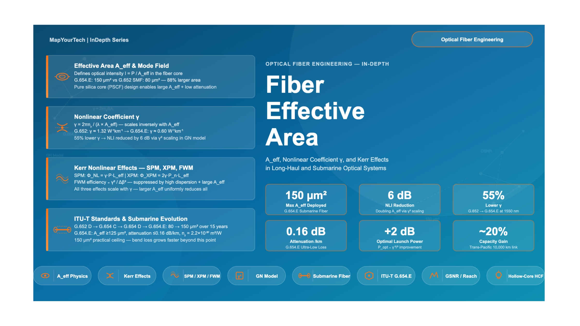
Fiber Effective Area and Its Impact on Nonlinearities

Last Updated: April 2, 2026

17 min read

Fiber Effective Area and Its Impact on Nonlinearities

Deep Dive | Optical Fiber Fundamentals

Fiber Effective Area and Its Impact on Nonlinearities

Section 1

Introduction

When engineers design a long-haul Dense Wavelength Division Multiplexing (DWDM) link or a submarine cable system, two fundamental limits define how much capacity can travel how far: amplifier noise and fiber nonlinearity. Amplifier noise — chiefly amplified spontaneous emission (ASE) from Erbium-Doped Fiber Amplifiers (EDFAs) — degrades the Optical Signal-to-Noise Ratio (OSNR). Fiber nonlinearity distorts signals through mechanisms that grow with optical intensity, ultimately corrupting the information carried on each wavelength channel. Managing both limits simultaneously is the central engineering challenge of modern optical transmission.

The fiber parameter that most directly governs how severe nonlinear distortion becomes is the effective area, A_eff. It represents the cross-sectional area over which the guided optical mode spreads inside the fiber core. A larger effective area means the same optical power is distributed over a wider region, reducing the optical intensity and thus suppressing the nonlinear interactions that degrade signal quality. This relationship is direct: doubling A_eff halves the optical intensity at any given launch power, and because most Kerr-based nonlinear effects scale with the square or cube of intensity, even modest increases in effective area produce substantial gains in system performance.

This article examines the physics of A_eff, the nonlinear coefficient γ (gamma), and the hierarchy of fiber standards that have evolved to deliver progressively larger effective areas — from standard single-mode fiber (SMF, ITU-T G.652) through the large effective-area designs of ITU-T G.654.E. It provides worked calculations, quantified comparisons, and practical design guidance drawn from long-haul terrestrial and submarine deployment experience, giving engineers the full picture needed to select and work with fiber types for today's high-capacity optical networks.

The discussion spans fiber mode theory, the Kerr effect and its manifestations as Self-Phase Modulation (SPM), Cross-Phase Modulation (XPM), and Four-Wave Mixing (FWM), the evolution of submarine fiber from 80 µm² to 150 µm² effective area, and the trade-offs that limit how large A_eff can practically become before bending loss and other physical constraints take over.

Section 2

What Is Fiber Effective Area?

2.1 Physical Definition

An optical fiber guides light by total internal reflection at the interface between a higher-refractive-index core and a lower-refractive-index cladding. In a single-mode fiber, only one transverse mode — the fundamental LP₀₁ mode — propagates. The intensity distribution of this mode across the fiber cross-section is approximately Gaussian: brightest at the center and decreasing toward the core–cladding boundary. The effective area quantifies the cross-sectional "size" of this intensity distribution using an energy-weighted average that captures how concentrated the optical field is.

Definition — Fiber Effective Area (Eq. 1)


           [ ∫∫ |E(x,y)|² dx dy ]²
  A_eff  =  ————————————————————————
            ∫∫ |E(x,y)|⁴ dx dy

Where:

A_eff — effective area of the fiber mode (units: µm²)

E(x,y) — transverse electric field amplitude of the guided mode at position (x, y)

The double integrals extend over the entire cross-section of the fiber.

Note: Because A_eff uses the square of the numerator and the fourth power of the field in the denominator, it heavily weights regions of high intensity. A fiber with light concentrated in a small bright spot will have a small A_eff, even if light technically extends into a larger area.

In practice, A_eff is closely related to — but not identical to — the Mode Field Diameter (MFD), which is more directly measurable. For a perfect Gaussian beam profile, the relationship is:

A_eff from Mode Field Diameter (Eq. 2)


             π × (MFD)²
  A_eff  ≈  —————————————
                  4

MFD — mode field diameter measured at the 1/e² intensity points (units: µm)

For G.652 SMF at 1550 nm: MFD ≈ 10.4 µm → A_eff ≈ 85 µm²

For G.654.E large-core fiber: MFD ≈ 13–14 µm → A_eff ≈ 130–150 µm²

Real fiber mode profiles deviate from a perfect Gaussian, so measured A_eff values from manufacturers are slightly different from the simple π×MFD²/4 approximation, but the formula gives a reliable first estimate and illustrates the key point: a wider mode means a larger effective area.

2.2 How Core Design Determines A_eff

Fiber manufacturers control A_eff primarily through the core radius and the refractive index contrast (the difference between core and cladding refractive indices, expressed as Δn or the normalized frequency V). A larger core radius spreads the mode over more cross-sectional area. A lower refractive index contrast also tends to push the mode further out (weakening the confinement), which expands the mode field.

The normalized frequency V is defined as:

Normalized Frequency V Parameter (Eq. 3)


          2π × a
  V  =  ———————————  × NA
             λ

  where  NA  =  √(n_core² − n_clad²)  ≈  n_core × √(2Δ)

a — core radius (µm)

λ — operating wavelength (nm)

NA — numerical aperture (dimensionless)

n_core, n_clad — core and cladding refractive indices

Δ — relative refractive index difference = (n_core − n_clad)/n_core

For single-mode operation: V must remain below approximately 2.405.

For a fiber to remain single-mode (V < 2.405) while also having a large A_eff, the designer must use a small Δn to compensate for any increase in core radius. This is exactly the approach used in pure silica core fibers (PSCFs) and extended pure silica core fibers (EPSCFs) that dominate modern submarine deployments. The germanium dopant used in standard G.652 fiber to raise the core refractive index is absent or minimized in these designs, which has the bonus of also reducing n₂ (the nonlinear refractive index), directly lowering fiber nonlinearity as an added benefit beyond the area increase.

Figure 1: Comparison of optical mode field intensity distribution between standard G.652 SMF and a large effective area G.654.E fiber. The expanded mode in the larger fiber reduces peak intensity significantly.

Section 3

The Nonlinear Coefficient γ and Its Relationship to A_eff

3.1 Defining γ

The nonlinear coefficient γ (gamma) is the single most important parameter for quantifying how much Kerr nonlinearity a fiber will produce per unit length per unit power. It combines the fiber's intrinsic material nonlinearity (captured by the nonlinear refractive index n₂) with the confinement of the mode (captured by A_eff) into one design-relevant number.

Nonlinear Coefficient (Eq. 4)


          2π × n₂
  γ  =  ————————————
           λ × A_eff

γ — nonlinear coefficient (W⁻¹km⁻¹)

n₂ — nonlinear refractive index of the fiber glass (m²/W); for pure silica: n₂ ≈ 2.2–2.7 × 10⁻²⁰ m²/W

λ — operating wavelength (m); typically 1550 nm = 1.55 × 10⁻⁶ m

A_eff — effective area (m²)

Key insight: γ scales inversely with A_eff. Doubling A_eff halves γ, directly halving the nonlinear distortion per unit length at the same power.

Worked Example: Standard SMF vs. G.654.E Fiber

Comparative Calculation (Eq. 5)


  Given: n₂(silica) = 2.6 × 10⁻²⁰ m²/W,   λ = 1550 nm

  G.652 SMF:   A_eff = 80 µm²  = 80 × 10⁻¹² m²
               γ = (2π × 2.6×10⁻²⁰) / (1.55×10⁻⁶ × 80×10⁻¹²)
               γ ≈ 1.32 W⁻¹km⁻¹

  G.654 fiber: A_eff = 150 µm² = 150 × 10⁻¹² m²
               γ = (2π × 2.2×10⁻²⁰) / (1.55×10⁻⁶ × 150×10⁻¹²)
               γ ≈ 0.60 W⁻¹km⁻¹

  Reduction in γ: (1.32 − 0.60) / 1.32 × 100 ≈ 55% lower nonlinearity

Premium Article — Free 20% Preview

Read the Full Analysis with Premium

The remaining 80% of this article — the design numbers, trade-offs and field guidance — is part of MapYourTech Premium, along with the full premium library, courses and professional tools.

View Membership Plans Already a member? Sign In

Instant access · Cancel anytime · 48-hour trial available

Sanjay Yadav

Optical Communications & Network Automation Expert | Author of 3 Books for Optical Engineers | Founder, MapYourTech

Optical networking engineer with nearly two decades of experience across DWDM, OTN, coherent optics, submarine systems, and cloud infrastructure. Founder of MapYourTech. Read full bio →

Follow on LinkedIn