
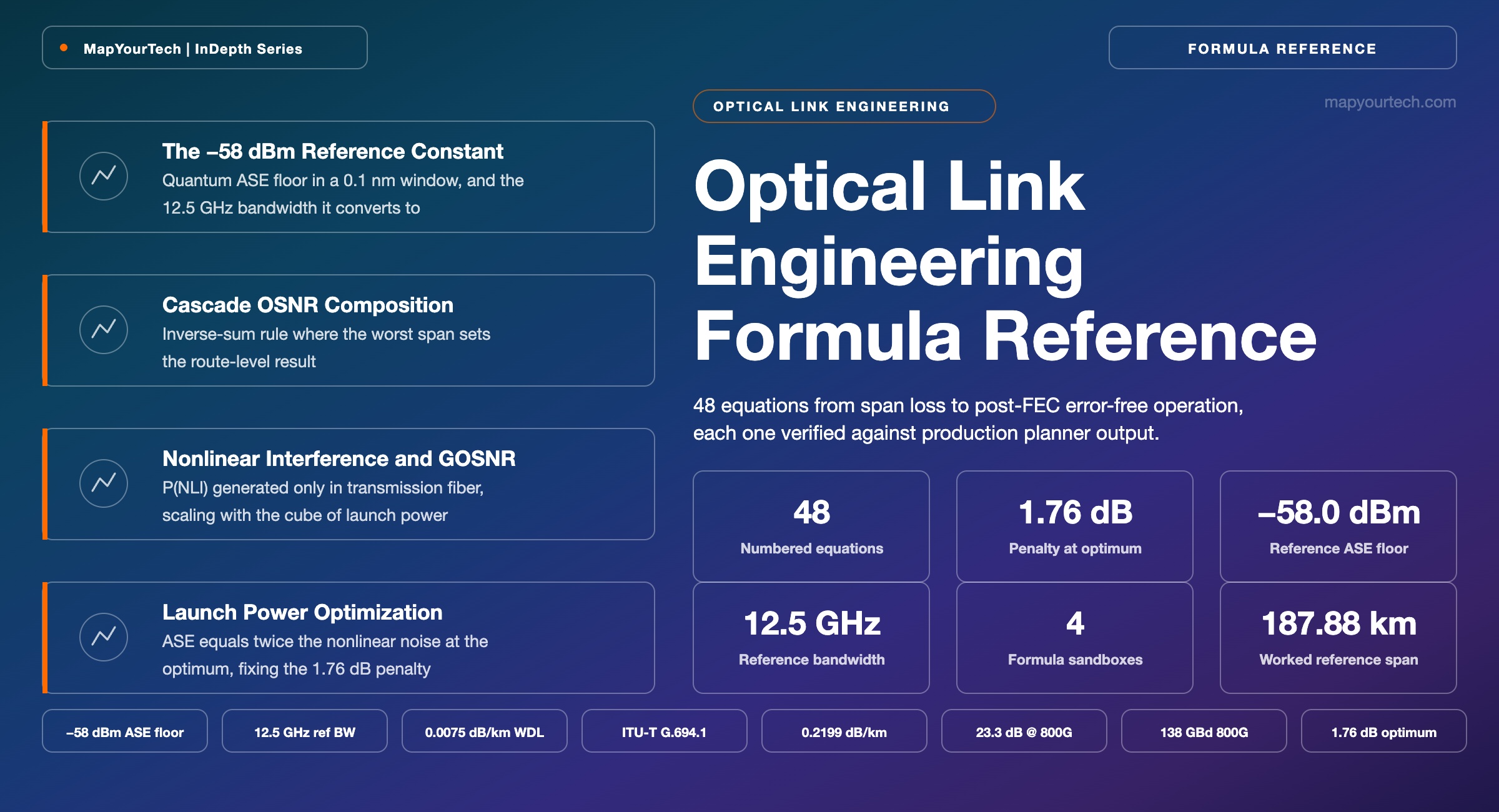
Optical Link Engineering Formula Reference: OSNR, GOSNR, Q-Factor and Launch Power Optimization
Every equation a DWDM planning tool evaluates between the transmitter and the FEC decoder, in the order it evaluates them — the −58 dBm reference constant, multi-stage noise composition, nonlinear interference generation and propagation, the four impairment penalty functions, the Q-factor and bit error rate mapping, and the launch power that maximizes generalized OSNR.
Every bit matters, but how you transmit them matters more.
Introduction
A DWDM planning tool that declares a lightpath feasible has evaluated roughly forty equations in a fixed order, and a planner who knows the order can tell within a minute which of them is the one that failed. The chain starts with a span loss and a launch power, converts them into an amplified spontaneous emission (ASE) noise floor through a single reference constant, adds a nonlinear interference term that scales with the cube of that same launch power, subtracts four penalty functions for chromatic dispersion, polarization mode dispersion, polarization dependent loss and nonlinear accumulation, and maps whatever margin survives onto a Q-factor and a pre-forward-error-correction bit error rate. Post-FEC error-free operation is a threshold test on the last number in that chain.
What makes the chain worth learning as a chain rather than as a set of independent formulas is that the same physical quantity appears in it three times with three different exponents. Per-channel launch power enters the ASE term linearly, so every decibel of extra power buys a decibel of optical signal-to-noise ratio (OSNR). It enters the nonlinear interference term cubically, so every decibel of extra power costs three decibels of nonlinear noise. And it enters the stimulated Raman scattering (SRS) tilt term through the total band power, so in a C+L system extra power in one band reshapes the spectrum of the other. Those three exponents fix the shape of every optimization decision in the rest of this reference, and they are also why extra launch power is worth taking only up to the point where the nonlinear term reaches half the ASE term.
This reference sets out each equation with its variable definitions and units, a worked numerical value, and a live sandbox where the equation has a clear input-to-output relationship worth experimenting with. The worked values are not illustrative: the single-span, cascade and submarine cases are carried end to end through the same chain a production planning tool applies, every intermediate value is reproducible from the stated inputs, and the Q-factor chain closes on its own reported Q-factor, Q-factor margin and pre-FEC bit error rate to three decimal places. Readers who want the noise accounting from first principles before the engineering forms should start with the OSNR fundamentals primer; readers who want the closed-form nonlinear theory behind the engineering approximations used here should read the Gaussian Noise model treatment.
Every number in this reference carries its provenance in the same sentence. Standard-specified values come from an ITU-T Recommendation or an equivalent published specification. Planner-computed values are the output of a production optical network planning tool for a measured route. Measured values come from optical time-domain reflectometer or optical spectrum analyzer characterization of that route. Theoretical limit values follow from information theory or from the closed-form nonlinear model. A figure without one of these labels is a definition, not a claim.
1. Reference Frame and the −58 dBm Constant
Optical signal-to-noise ratio is a ratio of two powers measured in different ways, and every disagreement between two tools that both report "OSNR" traces back to the reference bandwidth. The signal term is the total power of one channel. The noise term is the ASE power inside a fixed spectral window centred on that channel, conventionally 0.1 nm.
OSNR = PsignalPASE(Δνref) → OSNRdB = Psignal,dBm − PASE,dBm
Both powers in the same units. The noise term is bandwidth-dependent, the signal term is not — which is the entire source of reference-bandwidth confusion.
At 1550 nm the 0.1 nm window converts to an optical frequency span through the standard wavelength-to-frequency relation, and this conversion is the reason the number 12.5 GHz appears throughout coherent link engineering.
Δνref = c · Δλλ2 = (3 × 108) × (0.1 × 10−9)(1550 × 10−9)2 = 12.49 GHz
0.1 nm at 1550 nm equals 12.49 GHz, universally rounded to 12.5 GHz. Planning tools that use 12.48 GHz and tools that use 12.5 GHz differ by 0.007 dB — below any measurement threshold.
The ASE power spectral density at the output of an ideal amplifier is set by quantum mechanics, not by design choice, and evaluating it over the reference bandwidth produces a single constant that collapses all the physical constants into one number.
10·log10(h·ν·Δνref) = 10·log10(6.626×10−34 × 193.4×1012 × 12.48×109) = −58.0 dBm
Planck constant h in J·s, optical frequency ν at the C-band centre, reference bandwidth in Hz. Result expressed in dBm. Every OSNR estimate in the rest of this reference is built on this one number, and planning tools carry it internally as a base-noise constant of −58.
Because it is a quantum floor rather than an engineering parameter, the constant does not change with equipment or with route. It shifts marginally with band: evaluated at the L-band centre near 188.5 THz instead of 193.4 THz, the constant moves by 10·log10(188.5/193.4) = −0.11 dB, which production tools absorb rather than track. What does change is the third quantity in Eq. 3 when a receiver, not a spectrum analyzer, is the measuring instrument. A coherent receiver integrates noise over its own matched filter, whose noise bandwidth equals the symbol rate, so converting a spectrum-analyzer OSNR into the electrical signal-to-noise ratio a transceiver datasheet is written against requires an explicit bandwidth ratio.
OSNRdB = SNRdB + 10·log10Rs12.5 GHz
Rs is the symbol rate in GBd. A matched root-raised-cosine filter has a noise bandwidth of exactly Rs regardless of roll-off, so the roll-off factor β does not appear here. Roll-off enters only the occupied bandwidth Bocc = Rs·(1 + β), which sets channel spacing and the flexible-grid slot width, not the noise integration.
The practical size of that correction matters. A 138 GBd channel — the symbol rate of the 800 Gb/s line interfaces used in the worked cases later in this reference — carries a conversion term of 10·log10(138/12.5) = 10.4 dB. A receiver needing 12.9 dB of electrical SNR therefore needs 23.3 dB of measured OSNR, and that is exactly the threshold value the planning tool applies. Confusing the two domains produces a 10 dB design error, which is the single most expensive arithmetic mistake available in this discipline.
Takeaway: Three constants govern the whole reference frame: −58.0 dBm as the quantum ASE floor in a 0.1 nm window, 12.5 GHz as that window expressed in frequency, and 10·log10(Rs/12.5) as the bridge between optical OSNR and receiver SNR. Fix those three and every subsequent equation is arithmetic.
2. Span Loss, Wavelength-Dependent Loss and Channel Attenuation
Span loss is the input to everything downstream, and it is not one number per span but one number per channel. Silica attenuation falls across the C-band and rises again into the L-band, so the blue edge of the C-band arrives with measurably less power than the red edge after a long span. Planning tools model this as a linear tilt about the band centre rather than a full spectral curve.
αj = αref + WDL · (λj − λmid)Chmax / 2 αref = expected span lossL
WDL is the wavelength-dependent loss coefficient, 0.0075 dB/km in C-band planning practice. λj is the channel index on the ITU grid, λmid = 39 the centre channel index, Chmax = 88 the C-band channel count. αref is the measured average attenuation of the span in dB/km. Below 10 km the tilt term is dropped and αj = αref.
The corresponding L-band form replaces the ITU channel index with absolute frequency and normalises to the 4.8 THz L-band width, so the tilt term becomes FiberTilt · (fj − fmid,L) / (4.8 · L) with fmid,L = 188.475 THz. Channel power and the ASE noise accompanying it are then attenuated identically, which is why a passive span changes power levels without changing OSNR.
Pin(j) = P†(j) − αj·L Noisein(j) = Noise†(j) − αj·L
P† and Noise† are the values received from the upstream port, both in dBm; L is span length in km. Equal subtraction from both terms leaves OSNR unchanged — fiber loss degrades OSNR only indirectly, by forcing the amplifier that follows to work at a lower input power.
Read the Full Analysis with Premium
The remaining 89% of this article — the design numbers, trade-offs and field guidance — is part of MapYourTech Premium, along with the full premium library, courses and professional tools.
You May Also Like

-
Premium
-
August 18, 2026
-
Free
-
August 18, 2026

-
Free
-
August 18, 2026