
Gaussian Noise Model for Optical Transmission
Analytical Foundation, Closed-Form OSNR Calculation, Enhanced EGN Extension, and Application in Automated Network Planning Tools
Table of Contents
- Executive Summary
- Introduction & Background
- Historical Evolution
- Why "Gaussian"? — The Bell Curve Explained
- Physical Assumptions
- GN Model Formulation
- Enhanced EGN Model
- Multi-Span OSNR Calculation
- Network Planning Applications
- Validation & Accuracy
- Challenges & Limitations
- Future Directions
- Conclusion
- Glossary
- References
Executive Summary
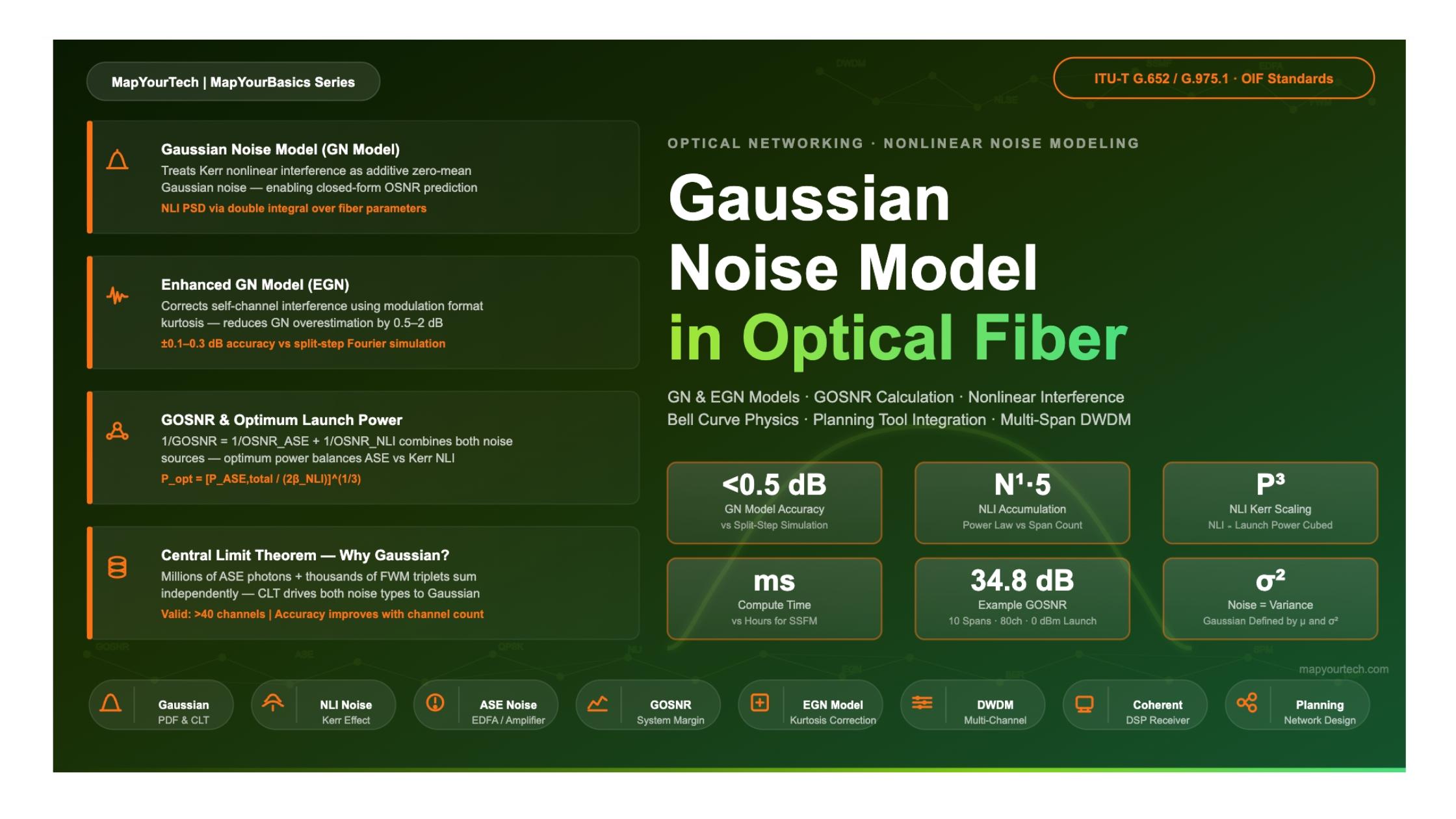
The Gaussian Noise (GN) model is an analytical framework that treats nonlinear interference (NLI) noise in multi-span, dense wavelength-division multiplexed (DWDM) optical transmission systems as additive, zero-mean Gaussian noise. By doing so, it enables engineers to compute the optical signal-to-noise ratio (OSNR) at the receiver in closed form, without resorting to computationally intensive time-domain or split-step Fourier simulations.
The model rests on three core physical assumptions: (1) the signal occupies a wide, spectrally flat bandwidth relative to the bandwidth over which Kerr-induced nonlinear interactions remain correlated; (2) dispersion is strong enough that walk-off between channels occurs over distances much shorter than a span length; and (3) the system operates in a pseudo-linear propagation regime. Under these conditions, the power spectral density (PSD) of the NLI noise contributed by each span can be expressed as a double integral over the channel frequencies, and the total NLI accumulates incoherently (in power) across spans.
The enhanced GN (EGN) model extends the basic formulation by correcting a systematic overestimation of self-channel interference (SCI) that arises when the signal modulation format deviates significantly from an ideal Gaussian distribution. For practical modulation formats such as quadrature phase-shift keying (QPSK) and 16-ary quadrature amplitude modulation (16-QAM), the EGN correction can amount to 0.5–2 dB in effective OSNR at typical operating points.
Both models have been validated against split-step simulations and field measurements. They form the analytical core of modern automated optical network planning tools, enabling rapid margin estimation, capacity forecasting, and spectral assignment for flex-grid systems. This article explains the physics, mathematics, implementation details, and engineering applications of the GN and EGN models in depth.
1. Introduction & Background
Why a closed-form noise model for fiber nonlinearity matters in modern network design
Modern long-haul DWDM transmission systems are jointly limited by two types of noise. The first is linear noise — principally amplified spontaneous emission (ASE) generated by erbium-doped fiber amplifiers (EDFAs) and other optical amplifiers placed at intervals along the route. The second is nonlinear noise — deterministic distortions arising from Kerr-effect interactions between co-propagating channels in the fiber. In practice, these two noise sources compete: increasing the per-channel launch power improves the ASE-limited signal-to-noise ratio but simultaneously intensifies nonlinear interference.
For system designers, quantifying both noise contributions accurately is essential for computing the generalized optical signal-to-noise ratio (GOSNR) or the effective signal-to-noise ratio (SNR) seen by the coherent receiver's digital signal processing (DSP) stack. The ASE contribution is straightforward: it follows directly from the amplifier gain, noise figure, and span count, using well-established cascade formulas. Nonlinear noise, by contrast, requires solving the nonlinear Schrödinger equation (NLSE) — or its generalizations — for the propagating waveform through each span, an inherently numerical task when many channels and many spans are involved.
The Gaussian Noise model resolves this computational bottleneck. Rather than tracking the evolution of each channel's electric field through each span, the GN model characterizes the aggregate nonlinear interference as an additive noise term whose power spectral density can be evaluated analytically. From an engineering perspective, this means that the total OSNR budget for a multi-span route can be computed in milliseconds, enabling automated network planning platforms to evaluate millions of candidate lightpath configurations in tractable time.
This article provides a self-contained treatment of the GN model: its physical motivation, its mathematical derivation in accessible form, the EGN extension, validation data, and practical guidance for deployment in network planning workflows. Engineers familiar with OSNR budgeting for ASE-limited systems will find that the GN and EGN models integrate naturally as an additional noise term alongside the ASE noise floor.
2. Historical Evolution of Nonlinear Noise Modeling
From time-domain simulation to closed-form analytical models
Understanding the progression of analytical tools for nonlinear noise provides essential context for appreciating what the GN model achieves and where its boundaries lie.
2.1 Early Per-Effect Approaches
The earliest system design tools treated each nonlinear effect — self-phase modulation (SPM), cross-phase modulation (XPM), and four-wave mixing (FWM) — as separate, independent penalty contributors expressed in dB. SPM caused spectral broadening and OSNR penalties that depended on launch power and span length. XPM introduced timing jitter and intensity fluctuations coupling between WDM channels. FWM generated parasitic tones at mixing frequencies that interfered with neighboring channels, a process particularly severe in low-dispersion fibers with regular channel spacing.
These per-effect formulas were analytically tractable but fundamentally incomplete. They could not capture the correlated interaction of all three mechanisms, nor could they predict how penalty contributions would combine under practical conditions of mixed modulation formats and non-uniform channel loading. System margins were consequently padded conservatively.
2.2 Split-Step Fourier Simulations
As computational resources improved through the 1990s and 2000s, the split-step Fourier method (SSFM) became the de facto standard for accurate system simulation. The SSFM numerically integrates the NLSE by alternately applying linear and nonlinear propagation operators over short fiber increments (steps). For a system with dozens of WDM channels, thousands of simulation symbols, and tens of spans, a single SSFM run can require hours to days of computation on high-performance hardware.
SSFM remains the benchmark for accuracy but is prohibitive for exhaustive network planning studies, which may need to evaluate millions of route-and-modulation-format combinations across a nationwide mesh topology. A faster analytical model was needed.
2.3 Birth of the Gaussian Noise Approximation
The observation that Kerr-induced distortions in highly dispersive, many-channel DWDM systems resemble additive Gaussian noise had been noted empirically for years. The insight that this observation could be formalized into a tractable analytical framework crystallized in a series of publications in the early 2010s. Researchers showed that when the DWDM signal ensemble is modeled as a spectrally shaped Gaussian noise process — the "GN approximation" — the perturbative solution to the NLSE yields a closed-form expression for the NLI power spectral density in terms of the channel powers, fiber parameters, span length, and number of spans.
This was a significant step forward: for the first time, a single analytical formula could predict the nonlinear noise floor of a multi-span DWDM system without simulation. Subsequent work refined the model to account for phase noise correlations across symbols — leading to the EGN model — and extended its applicability to flex-grid, rate-adaptive coherent systems.
3. Why "Gaussian"? — The Name, the Shape, and What It Means for Optical Engineers
Understanding what the Gaussian distribution is, what the bell curve shows, and exactly why it applies to noise in optical fiber
The word "Gaussian" appears in dozens of optical engineering terms — Gaussian beam, Gaussian pulse, Gaussian noise, Gaussian filter — and they all trace back to the same mathematical function, named after the German mathematician Carl Friedrich Gauss (1777–1855). Understanding what the function describes, why it arises so naturally in physics, and why optical fiber noise specifically takes this shape is essential context before diving into the GN model's formulas.
3.1 What is a Gaussian Distribution?
A Gaussian distribution — also called the normal distribution — is a continuous probability distribution that describes how the values of a random variable are spread around a central mean. It is defined by just two parameters: the mean (μ), which sets the center of the distribution, and the standard deviation (σ), which sets how wide or narrow the spread is. The probability density function (PDF) is:
p(x) = 1 / (σ √(2π)) × exp[ -(x - μ)² / (2σ²) ]
| Symbol | Meaning | Physical Meaning in Optical Noise |
|---|---|---|
| p(x) | Probability of observing value x | Probability that noise amplitude takes value x at an instant |
| μ (mu) | Mean — the center of the distribution | For noise: μ = 0 (noise has zero average — it has no DC component) |
| σ (sigma) | Standard deviation — width of spread | Related to noise power: P_noise = σ² (variance = power for zero-mean noise) |
| σ² | Variance | Equals the total noise power in the signal |
| exp(…) | Exponential decay term | Creates the bell shape — values far from center are very unlikely |
Two features of this equation define the bell curve's characteristic shape. The exponent is always negative (since it involves a squared term divided by a positive number), so p(x) is always positive and always decreasing as x moves away from μ. The exponential decay is symmetric around μ, which is why the bell curve is perfectly symmetric. The denominator term σ√(2π) normalizes the total area under the curve to exactly 1, as any valid probability distribution must satisfy.
3.2 Anatomy of the Bell Curve — What Every Part Means
3.3 Why Does Optical Fiber Noise Follow a Gaussian Distribution?
This is the key question: why does noise in an optical system — whether ASE from amplifiers or NLI from the fiber Kerr effect — end up with this specific bell-curve shape, rather than some other distribution like uniform noise or Poisson noise? There are two separate physical reasons, one for each noise type.
3.3.1 ASE Noise Is Gaussian — The Central Limit Theorem
Amplified spontaneous emission is generated when electrons in the erbium-doped fiber return spontaneously from an excited energy state to the ground state, emitting photons at random times and random phases. Each spontaneous emission event is independent, and each contributes a tiny complex-valued electric field fluctuation to the propagating signal. The total ASE field at any instant is the sum of an enormous number of these independent, random, small-amplitude contributions.
This is precisely the scenario described by the Central Limit Theorem (CLT): when you add a large number of independent random variables — regardless of what distribution each individual variable follows — the sum approaches a Gaussian distribution. The ASE field amplitude at any frequency has real and imaginary parts that each independently follow Gaussian statistics. The ASE power, which is proportional to the squared magnitude of the field, follows a chi-squared distribution, but for the purposes of the GN model, it is the field (not power) that is modeled as Gaussian, and the field noise is what the DSP receiver processes.
The Central Limit Theorem in Practice — A Physical Analogy
Imagine a fiber amplifier containing millions of erbium ions. Each ion may emit a spontaneous photon independently. No single ion controls the noise — the noise is the collective result of all of them acting at once. Just as the average height of a large group of people follows a bell curve even though individual heights do not strictly follow any simple distribution, the sum of all spontaneous emissions becomes Gaussian. In a 1 nm bandwidth at 1550 nm, a typical EDFA generates roughly 107 spontaneous photons per second — more than enough for the Gaussian approximation to be essentially exact.
3.3.2 NLI Noise Is Gaussian — Four-Wave Mixing of Many Channels
The Gaussian nature of NLI has a different origin. Nonlinear interference arises from four-wave mixing between all triplets of frequency components in the DWDM signal. Each triplet generates a mixing product at a new frequency. When a DWDM system carries 40, 80, or 200 channels — each independently modulated — there are an enormous number of such triplets mixing simultaneously at any given frequency in the spectrum. Each mixing product has a random phase and amplitude determined by the instantaneous data patterns on the contributing channels.
Once again, the Central Limit Theorem applies: the NLI field at a given frequency is the sum of a large number of statistically independent, small-amplitude mixing products. That sum approaches a Gaussian distribution. The more channels the system carries, the more mixing triplets contribute, and the better the Gaussian approximation holds. For 4 channels, the approximation is rough. For 80 channels, it is excellent.
ASE Noise — Why Gaussian
- Generated by millions of independent spontaneous emission events per second
- Each emission: random phase, random time
- Sum of many independent randoms → Central Limit Theorem → Gaussian
- Zero-mean: no average field component, only fluctuations
- Power = σ²: scales with amplifier NF and gain
- Holds exactly for any number of channels
NLI Noise — Why Gaussian (GN Approximation)
- Generated by FWM triplets among all DWDM channel pairs
- Each triplet: random amplitude determined by modulated data
- Sum of many triplets → Central Limit Theorem → Gaussian
- Accuracy increases with channel count
- Power = σ² ∝ Pch³ (Kerr-cubic dependence)
- EGN correction needed for few channels or non-Gaussian constellations
3.4 What Different Bell Curve Shapes Mean for System Performance
The bell curve's shape directly determines whether a transmission system meets its bit error rate (BER) target. The key insight is this: the signal is located at a fixed amplitude level, and the noise forms a bell curve around zero. A bit error occurs when the noise amplitude is large enough to push the received signal past the decision threshold. The probability of this happening is determined by how much of the bell curve's tail extends beyond the decision boundary.
A narrow bell curve (small σ, low noise power, high OSNR) keeps almost all noise samples close to zero. The tails are extremely thin, and the probability of a noise fluctuation large enough to cause a bit error is vanishingly small — for example, a Q-factor of 7 corresponds to a BER of 10-12, meaning only 1 in a trillion bits is in error, because the curve's tails at ±7σ from the mean contain only that tiny fraction of the area. A wide bell curve (large σ, high noise power, low OSNR) has fat tails: a significant fraction of noise samples are large enough to cross the decision boundary and cause errors.
This explains directly why the OSNR threshold exists for each modulation format: higher-order modulation (16-QAM, 64-QAM) packs signal constellation points closer together, reducing the effective distance from each symbol to the nearest decision boundary. A noise fluctuation only needs to be half as large to cause an error, so the bell curve must be narrower (higher OSNR) to achieve the same BER. Specifically, doubling the constellation density roughly doubles the required OSNR in linear terms — approximately a 3 dB requirement increase per factor-of-2 increase in modulation order.
3.5 A Summary: The Three Properties That Make Gaussian Noise Special
Completely Described by Two Numbers
A Gaussian distribution is fully characterized by just its mean μ and its variance σ². For optical noise, μ = 0 (zero-mean) and σ² = noise power. This means that knowing PASE and PNLI completely describes the noise statistics — no further information is needed. This is what makes the GN model powerful: computing those two numbers suffices for full performance prediction.
The Sum of Gaussians Is Gaussian
If ASE noise is Gaussian with variance σASE² and NLI noise is Gaussian with variance σNLI², then their sum is also Gaussian with variance σASE² + σNLI². This additive property means the total noise power is simply the sum of ASE and NLI powers — the basis of the GOSNR formula. No complex probability distribution arithmetic is needed.
Direct Link to BER via the Q-Function
For Gaussian noise, the BER is exactly computable using the Q-function (the complementary error function): BER = Q(σnoise/d), where d is the distance from the signal to the decision boundary. This closed-form relationship is what allows coherent receiver DSP performance curves to be computed analytically from GOSNR, without requiring simulation of the entire detection chain.
4. Physical Assumptions Behind the GN Model
What must be true for the Gaussian approximation to hold — and when it breaks down
The GN model rests on three interrelated physical assumptions. Understanding each assumption — including the conditions under which it holds and where it breaks down — is essential for applying the model correctly in practical system design.
3.1 The Gaussian Signal Approximation
The central assumption is that the aggregate DWDM signal at any point in the fiber can be modeled as a zero-mean, wide-sense stationary Gaussian random process with a power spectral density equal to the sum of the individual channel spectra. This approximation becomes increasingly accurate as the number of DWDM channels increases, because the superposition of many independently modulated channels tends toward Gaussian statistics by the central limit theorem. For a system with 40 or more channels at Nyquist spacing, the Gaussian approximation is generally excellent.
For a small number of channels, or for channels whose modulation format imposes a very non-Gaussian amplitude distribution (such as on-off keying with high extinction ratio, or highly probabilistically shaped QAM), the approximation degrades. The EGN model explicitly accounts for the deviation of the channel statistics from Gaussian through a correction factor dependent on the modulation format's fourth-order moment (kurtosis).
3.2 Strong Dispersion and Incoherent NLI Accumulation
The second assumption concerns the role of chromatic dispersion in the NLI process. In standard single-mode fiber (SSMF), the dispersion coefficient is approximately 17 ps/(nm·km) in the C-band. This large dispersion causes different spectral components of the DWDM signal to walk through one another on a length scale called the walk-off length, which for typical channel spacings and symbol rates is on the order of a few kilometers — far shorter than a typical span length of 80–100 km.
Because NLI is generated by phase-matched interactions between frequency components, and because high dispersion disrupts phase matching rapidly, the NLI generated in one segment of the span is largely uncorrelated with NLI generated in a different segment. Similarly, NLI accumulated in different spans adds incoherently in power (rather than coherently in field amplitude). This incoherent accumulation is what makes the GN model's closed-form expressions possible: the total NLI power over N identical spans is simply N times the single-span NLI power (with a weak correction factor depending on the number of spans).
This assumption is well justified for SSMF but is violated for dispersion-shifted fiber (DSF, ITU-T G.653), where the dispersion is near zero at 1550 nm, and is also less accurate for non-zero dispersion-shifted fiber (NZDSF, ITU-T G.655) with low dispersion coefficients. In those cases, phase matching over longer distances can cause NLI to accumulate more coherently (quasi-coherently), leading to N² or N^(1.5+ε) scaling rather than the N^1.5 behavior characteristic of the GN model for fully incoherent accumulation.
3.3 First-Order Perturbation Theory
The third assumption is that the Kerr nonlinearity acts as a small perturbation on the linear propagation. The GN model's derivation uses first-order perturbation theory applied to the NLSE: the signal field is written as the sum of a linear part (which would propagate without nonlinearity) and a small nonlinear correction. The NLI power is computed from this first-order correction. Higher-order terms (second-order perturbation, etc.) are neglected.
This assumption holds well when the nonlinear phase accumulation per span — often characterized by the nonlinear phase shift parameter φNL = γ P Leff, where γ is the fiber nonlinear coefficient, P is the launch power, and Leff is the effective length — is much less than 1 radian. For typical long-haul systems with launch powers near the optimum, φNL per span is typically in the range 0.05–0.3 rad, which is well within the perturbative regime. Near the maximum useful launch power, higher-order effects become more important, and the GN model begins to underestimate the true NLI.
4. GN Model Formulation
The closed-form expression for NLI power spectral density and its engineering simplifications
4.1 The NLSE and Perturbative Approach
Signal propagation in a single-mode optical fiber is governed by the generalized NLSE. Neglecting polarization effects and higher-order dispersion terms, the equation for the slowly varying field envelope A(z, t) is:
∂A/∂z = -(α/2)A - j(β2/2) ∂²A/∂t² + jγ|A|²A
| Symbol | Meaning | Typical Value |
|---|---|---|
| A(z,t) | Slowly varying complex field envelope | — |
| α | Power attenuation coefficient | 0.046 km⁻¹ (0.2 dB/km) |
| β2 | Group-velocity dispersion (GVD) coefficient | −21.7 ps²/km (SSMF, C-band) |
| γ | Nonlinear coefficient | 1.3 (W·km)⁻¹ (SSMF) |
| j | Imaginary unit | — |
In the GN model, the field A is decomposed as A = A0 + a1, where A0 is the linear solution (propagating as if γ = 0) and a1 is the first-order nonlinear perturbation. Substituting into the NLSE and retaining only first-order terms in γ yields a driven linear equation for a1 whose source term involves the Kerr-induced mixing products of A0.
4.2 The NLI Power Spectral Density — Single Span
After solving the perturbation equation in the frequency domain and computing the power spectral density of the resulting first-order NLI field, one arrives at the core GN model expression for the NLI noise PSD generated in a single fiber span of length Ls:
GNLI(f)  =  (16/27) γ²
         ∞    ∞
         ∫    ∫   G(f1) G(f2) G(f1+f2-f)
        -∞   -∞
         ×  |ρ(f1, f2, f, Ls)|²  df1 df2
| Symbol | Meaning |
|---|---|
| G(f) | PSD of the total DWDM signal (sum of all channel spectra) |
| γ | Fiber nonlinear coefficient [(W·km)⁻¹] |
| 16/27 | Polarization factor for dual-polarization coherent systems |
| ρ(f₁, f₂, f, Ls) | Nonlinear phase-matching kernel accounting for dispersion and attenuation |
| f₁, f₂ | Integration frequency variables |
The kernel ρ encapsulates the interplay between Kerr nonlinearity, chromatic dispersion, and fiber loss. Its squared magnitude, evaluated at a given output frequency f, represents the efficiency with which a triad of input frequency components at f₁, f₂, and f₁+f₂−f interact to deposit NLI noise at f. For large dispersion, |ρ|² falls off rapidly as |f₁−f| and |f₂−f| increase, confining significant NLI contributions to nearby frequencies and justifying the "local" character of the nonlinear interaction.
4.3 Multi-Span Extension
For a chain of N identical spans — each with the same fiber type, length, launch power, and amplifier gain perfectly compensating for span loss — the total NLI PSD at the receiver is the incoherent sum over all spans:
GNLI,total(f) = N × GNLI,span(f)
This linear scaling holds when NLI from different spans accumulates incoherently (strong dispersion condition). For partially coherent accumulation (low-dispersion fiber), the scaling approaches N² for fully coherent addition.
For a system with non-identical spans (different lengths, fiber types, or launch powers), the total NLI is the sum of each span's individual contribution — a straightforward extension that modern planning tools implement.
4.4 The Integrated GN Formula and Closed-Form Approximation
The double integral in Equation 2 can be evaluated numerically for any channel loading scenario. For the special case of a flat-spectrum, uniform channel comb occupying a total bandwidth BWDM, an approximate closed-form solution can be derived by assuming rectangular channel spectra and approximating the kernel integration:
PNLI  ≈  (16/27) γ² Pch³ Leff²
           × (Nch² - 1) Δf²   /* cross-channel (XCI) term */
           ×  f(β2, Ls, Rs)      /* dispersion-dependent factor */
           ×  N                   /* number of spans */
| Symbol | Meaning |
|---|---|
| Pch | Per-channel launch power [W] |
| Leff | Effective nonlinear length: Leff = (1 − e−αLs) / α |
| Nch | Number of DWDM channels |
| Δf | Channel spacing [Hz] |
| f(β₂, Ls, Rs) | Dispersion-dependent factor involving arcsinh or logarithm |
| N | Number of fiber spans |
The dominant dependence of PNLI on system parameters can be read off directly from this expression: NLI power scales as Pch3 (cubic in launch power), as Leff2 (proportional to effective length squared), and as N (linearly in span count for fully incoherent accumulation). These scaling laws have been confirmed extensively against split-step simulations and form the basis for understanding the optimal launch power that maximizes OSNR, as discussed in Section 7.
Key Points — GN Model Formulation
- NLI noise PSD is expressed as a double frequency-domain integral of the signal PSD convolved with itself and the dispersion kernel.
- For N identical spans with strong dispersion (SSMF), total NLI accumulates as N × PNLI,span — linear in span count.
- PNLI ∝ Pch3: a 1 dB increase in launch power increases NLI by 3 dB.
- The 16/27 prefactor arises from averaging Kerr interactions over both polarizations in a dual-polarization coherent system.
- Closed-form approximations enable millisecond-timescale OSNR computation for automated planning tools.
5. The Enhanced GN (EGN) Model
Correcting for modulation-format-dependent self-channel interference
5.1 The GN Model's Key Limitation
The GN model's Gaussian signal assumption overestimates a specific component of NLI called self-channel interference (SCI) — the nonlinear crosstalk that a channel imposes on itself. For a truly Gaussian-distributed signal, SCI has a specific relationship to XCI (cross-channel interference) and multi-channel interference (MCI). Real modulation formats, however, have different statistical moments from a Gaussian distribution. The ratio of the fourth-order moment to the square of the second-order moment — the kurtosis — differs from the Gaussian value of 3.
For QPSK, the symbols form a unit circle constellation, and the amplitude is constant. The kurtosis of the QPSK amplitude distribution is lower than Gaussian. This means the GN model overestimates SCI for QPSK, because SCI arises from the amplitude fluctuations of the signal interacting with itself, and QPSK has less amplitude fluctuation than Gaussian noise. For 16-QAM, the situation is intermediate between Gaussian and QPSK. The GN model's systematic overestimation of SCI translates into a pessimistic (conservative) NLI estimate.
5.2 The EGN Correction Term
The EGN model adds a correction to the GN model's NLI power that accounts for the non-Gaussian nature of the signal. The correction is expressed in terms of the fourth-order cumulant (excess kurtosis) of the signal's probability distribution:
PNLI,EGN  =  PNLI,GN  +  ΔPNLI,SCI

ΔPNLI,SCI  =  (κch - 1)  ×  CSCI  ×  Pch³
| Symbol | Meaning |
|---|---|
| PNLI,GN | NLI power from standard GN model |
| κch | Normalized fourth-order moment of channel symbols (= 1 for Gaussian) |
| CSCI | SCI coefficient (involves fiber parameters and span geometry) |
| κch = 1 for Gaussian | → correction = 0 (GN model exact) |
| κQPSK ≈ 1/2 | → correction is negative (GN overestimates NLI) |
| κ16-QAM ≈ 0.68 | → smaller negative correction |
Because the correction term for QPSK is negative (the GN model overestimates NLI for QPSK), the EGN model predicts a lower NLI than GN, translating to a higher OSNR margin. The practical implication is that using the GN model for system design with QPSK modulation is conservative — it leaves unallocated margin that could be used to extend reach or increase data rate. However, in margin-critical scenarios (e.g., submarine systems operating near the limit), the EGN correction can make the difference between a viable and a non-viable design.
GN Model — When to Use
- Rapid preliminary OSNR estimation for large network studies
- Systems with high modulation orders (64-QAM, 256-QAM) approaching Gaussian statistics
- When conservative (pessimistic) margin estimates are preferred
- Automated planning tools requiring millisecond computation time
- Fully loaded WDM systems with many channels
EGN Model — When to Use
- Detailed design studies where accurate NLI prediction matters
- QPSK and 16-QAM systems (GN overestimation is most significant)
- Margin-critical links such as submarine or ultra-long haul
- Probabilistically shaped QAM with non-standard kurtosis
- Validating GN-based planning tool results
6. Multi-Span OSNR Calculation Using the GN Model
Integrating ASE and NLI noise contributions into a total system OSNR budget
6.1 Total OSNR — Combined Noise Budget
In a multi-span optically amplified system, the total degradation in signal quality at the receiver results from the combined effect of ASE noise accumulated over all amplifiers and NLI noise accumulated over all fiber spans. Both noise sources are modeled as additive Gaussian noise in the GN framework, so their contributions to the total noise power simply add. This leads to the following expression for the total OSNR:
GOSNRtotal⁻¹  =  OSNRASE⁻¹  +  OSNRNLI⁻¹

Where:
OSNRASE  =  Pch  /  (N  ×  PASE,span)

OSNRNLI  =  Pch  /  PNLI,total

PASE,span  =  nsp  (G-1)  hf  Bref   /* B_ref = 12.5 GHz */
| Symbol | Meaning |
|---|---|
| N | Number of spans |
| nsp | Spontaneous emission factor (= NF/2 for saturated EDFA) |
| G | Amplifier gain (linear) |
| h | Planck's constant (6.626×10⁻³⁴ J·s) |
| f | Optical carrier frequency |
| Bref | Reference bandwidth, typically 12.5 GHz (0.1 nm at 1550 nm) |
The generalized OSNR (GOSNR) is the figure of merit used by modern coherent receiver DSP chains. It differs from the traditional OSNR definition (which considers only ASE in a 0.1 nm bandwidth) in that it integrates the noise over the actual channel bandwidth and includes NLI. The GOSNR is directly related to the effective SNR seen by the forward error correction (FEC) decoder.
6.2 Optimum Launch Power
The dependence of GOSNR on per-channel launch power Pch exhibits a characteristic bell-shaped curve (on a log-log scale). At low launch powers, GOSNR is dominated by ASE noise and improves as Pch increases. At high launch powers, NLI dominates and GOSNR decreases as Pch increases (since PNLI ∝ Pch3). The peak occurs at the optimum launch power Popt:
Popt  =  [ PASE,total  /  (2 βNLI) ]1/3

Where:
βNLI  =  PNLI,total / Pch³   /* NLI coefficient */

GOSNRmax  =  (3/2) Popt / PASE,total
At Popt, the NLI noise power is exactly half the ASE noise power (the ratio OSNRASE/OSNRNLI = 2 at the optimum). The peak GOSNR is 1.76 dB higher than the OSNR at the same launch power in an ASE-only system, because the optimal balance of ASE and NLI slightly favors operating with some NLI present.
Multi-Span GOSNR Calculation — 10-Span C-Band System
Consider a 10-span SSMF system with the following parameters:
- Span length: Ls = 80 km; Fiber attenuation: α = 0.2 dB/km
- Amplifier noise figure: NF = 5 dB; EDFA gain G = 16 dB (compensates span loss)
- Number of channels: Nch = 80; Channel spacing: Δf = 50 GHz
- Per-channel launch power: Pch = 0 dBm = 1 mW
- Fiber nonlinear coefficient: γ = 1.3 (W·km)⁻¹; Dispersion: D = 17 ps/(nm·km)
The result of GOSNR ≈ 34.8 dB is dominated by ASE noise at this launch power (0 dBm). For 100G QPSK channels requiring approximately 13–15 dB OSNR (in channel bandwidth), the system has ample margin. For 400G 16-QAM channels requiring ~21–23 dB GOSNR in channel bandwidth, a narrower margin remains after accounting for DSP penalties.
7. Application in Automated Network Planning Tools
How GN and EGN models are integrated into software-defined planning and margin estimation
The computational efficiency of the GN model — and its EGN refinement — makes it the natural choice as the nonlinear noise engine in automated optical network planning tools. These tools must evaluate millions of lightpath configurations across complex mesh topologies, selecting modulation formats, baud rates, and spectral slots that maximize throughput while maintaining adequate margin. Without an analytical model for NLI, this optimization would require SSFM calls for every candidate configuration, making it computationally intractable.
7.1 The Planning Tool Workflow
Network Topology and Link Parameter Ingestion
The tool ingests a network topology database containing span lengths, fiber type (SSMF, NZDSF, submarine low-loss fiber), attenuation coefficients, dispersion profiles, amplifier locations, gain values, and noise figures. For flex-grid systems, the amplifier gain tilt and gain flatness may also be characterized.
Per-Lightpath GOSNR Estimation
For each candidate lightpath (defined by its source/destination nodes, spectral slot, modulation format, and baud rate), the tool computes the accumulated ASE using cascade noise figure formulas and the accumulated NLI using the GN or EGN model, integrated numerically over the actual channel loading and spectrum assignment. The resulting GOSNR is compared against the receiver's required SNR threshold for the selected modulation format and FEC scheme.
Margin-Aware Modulation Format Selection
With a rapid GOSNR estimate available for each candidate configuration, the tool selects the highest-order modulation format (and corresponding maximum baud rate) whose required SNR can be met with a defined margin (typically 2–3 dB system margin). This is the core of adaptive bitrate or rate-adaptive coherent transponder configuration.
Spectrum Assignment and Optimization
NLI is spectrally non-uniform: channels at the center of the DWDM band experience more XCI from channels on both sides, while edge channels receive contributions from only one side. The planning tool uses the GN model's frequency-resolved output to account for this spectral variation, enabling informed spectrum assignment that places the most sensitive channels (highest modulation order) in spectral positions with the lowest NLI.
Launch Power Optimization
Using the GN model's prediction of optimum launch power (Equation 7), the tool can recommend or automatically configure per-channel launch powers that maximize GOSNR. In heterogeneous systems with mixed modulation formats and rates, the optimum power may vary per channel, and the tool balances NLI minimization against the risk of EDFA spectral distortion from non-flat power loading.
7.2 GN Model in Open and Disaggregated Networks
The rise of open, disaggregated optical networking — where the optical line system (amplifiers, ROADMs, fiber) and the transponders may come from different vendors — has intensified the need for accurate, vendor-agnostic OSNR models. The GN model, parameterized by measured fiber and amplifier characteristics, provides exactly this: a common analytical framework that can be populated with measured parameters from any vendor's equipment.
Open optical transport standards bodies including OIF (Optical Internetworking Forum) have contributed to standardizing the information model for expressing GN-model parameters — such as span loss, fiber type, and amplifier noise figure — enabling interoperability between different planning tools and network equipment management systems (EMS/NMS). The GN model thus serves as the analytical bridge between the physical-layer characterization data provided by equipment vendors and the capacity planning algorithms running in the network controller.
8. Validation and Accuracy Assessment
How GN and EGN model predictions compare to simulation and experiment
8.1 Comparison Against Split-Step Simulations
The GN model has been extensively validated against SSFM simulations across a range of system configurations. For large channel counts (32 or more channels) on SSMF with optimum or near-optimum launch power, the GN model typically agrees with SSFM to within 0.5 dB in predicted NLI noise power — excellent accuracy for an analytical model. The agreement is tightest for systems with high dispersion, many channels, and uniform channel loading.
Deviations between the GN model and SSFM are most pronounced under the following conditions. First, for systems with very few channels (2–4), the Gaussian signal assumption is poorly justified and the GN model can overestimate NLI by 1–2 dB. Second, for very low channel count combined with QPSK or other constant-envelope modulation, the EGN correction is large and the basic GN model is notably pessimistic. Third, for systems operating significantly above the optimum launch power (nonlinear phase shift >> 0.3 rad/span), higher-order perturbative contributions become important and the GN model underestimates distortion.
8.2 Experimental Validation
Laboratory and field measurements have confirmed the GN model's predictions. Transmission experiments over installed fiber plant — where fiber parameters are well characterized — have demonstrated that the GN model predicts the measured Q-factor within 0.3–0.5 dB margin for standard long-haul SSMF routes carrying 100G or 400G coherent channels. Discrepancies beyond this range are typically attributable to polarization mode dispersion (PMD), laser phase noise contributions, or incomplete characterization of the fiber's dispersion profile and nonlinear coefficient along the route.
| Attribute | GN Model | EGN Model | Split-Step SSFM |
|---|---|---|---|
| Computation time (80 channels, 10 spans) | ~1 ms | ~5 ms | ~1–10 hours |
| Accounts for modulation format statistics | No (Gaussian assumed) | Yes (kurtosis correction) | Yes (exact) |
| Accuracy vs SSFM (many channels, SSMF, optimum power) | ±0.3–0.5 dB | ±0.1–0.3 dB | Reference |
| Handles non-uniform spectrum loading | Yes (numerical integration) | Yes | Yes |
| Valid for low-dispersion fiber (NZDSF, DSF) | Limited (quasi-coherent accumulation not captured) | Limited | Yes |
| Suitable for automated network planning | Yes (primary choice) | Yes (with some extra compute) | No (too slow) |
| Captures high-order nonlinearity (solitons, FWM cascades) | No | No | Yes |
| Validated for 100G–400G coherent DWDM | Yes | Yes | Yes |
9. Challenges and Limitations
Where the GN model requires care and how engineers work around its boundaries
9.1 Low-Dispersion Fiber Regimes
The GN model's assumption of incoherent NLI accumulation breaks down for low-dispersion fiber, where NLI from different spans can add quasi-coherently. For submarine cable systems employing ultralow-loss, low-nonlinearity fiber, or for terrestrial links still running older non-zero DSF, the NLI scaling may lie between the N (fully incoherent) and N² (fully coherent) limits. In these cases, a phased-array or quasi-coherent correction factor must be applied to the GN model prediction, or a fully numerical integration is required.
9.2 Non-Uniform Channel Loading and Spectral Hole Burning
Real networks frequently operate with non-uniform channel loading — some spectral slots occupied, others empty. The GN model's double integral formulation can accommodate this by using the actual channel PSD profile, but the presence of spectral gaps significantly modifies the NLI distribution. Channels adjacent to an empty spectral slot experience reduced XCI from that direction. Planning tools must therefore account for the specific channel loading configuration, not just the total optical power.
EDFA gain dynamics also interact with channel loading. In a partially loaded system, the EDFA may allocate more gain to the occupied channels, changing the per-channel power relative to the fully loaded case and requiring an updated GN model input. Accurate planning therefore requires a joint model of amplifier gain tilt and NLI noise.
9.3 Polarization and PMD Effects
The GN model, in its standard form, treats both polarization modes as equally loaded and fully de-correlated over distances longer than the polarization beat length. This is accurate for the average NLI prediction in standard SSMF but does not capture the instantaneous NLI variation due to PMD-driven polarization rotation. For systems with significant PMD, the NLI noise exhibits additional fluctuations beyond the GN model's average prediction. Coherent receiver DSP generally handles these fluctuations through adaptive polarization demultiplexing, but the NLI model should account for the average correctly.
9.4 Stimulated Raman Scattering in Wideband Systems
As DWDM systems expand into wideband configurations spanning both the C-band and L-band (200 nm total optical bandwidth), stimulated Raman scattering (SRS) causes systematic power tilt from shorter-wavelength channels to longer-wavelength channels. This power tilt modifies the effective per-channel launch power seen by the NLI process, requiring the GN model to be coupled with an SRS model. For ultra-wideband systems covering more than 40–50 nm of optical bandwidth, neglecting SRS can lead to significant errors in the predicted NLI distribution across the band.
10. Future Directions
Extending analytical NLI models to meet emerging system challenges
Several research directions are extending the GN and EGN model frameworks to address the limitations described above and to meet the requirements of next-generation systems.
Wideband GN models that incorporate Raman-induced power tilt are an active research area. By coupling the SRS power transfer equation with the GN NLI integral, researchers have developed analytical models that predict the NLI PSD across the full C+L band, enabling accurate capacity planning for wideband systems. These extended models have been validated against SSFM for bandwidths up to 12 THz, showing good agreement when SRS is properly accounted for.
Machine learning augmentation of the GN model addresses scenarios where the analytical assumptions are violated — for example, in deployed networks with partially unknown fiber parameters. Neural network models trained on simulation data can provide correction factors that bring the GN model's predictions closer to ground truth for unusual fiber profiles, thereby extending the model's applicability without full numerical simulation.
Probabilistic shaping (PS) is becoming standard in high-performance coherent transponders. PS modifies the probability distribution of transmitted symbols to approach a Maxwell-Boltzmann distribution, maximizing the shaping gain over the AWGN channel. The EGN model can be extended to handle PS by computing the modified kurtosis of the shaped constellation, but research is ongoing to develop computationally efficient closed-form expressions for the PS-EGN correction factor across the range of shaping parameters used in practice.
Real-time NLI monitoring and closed-loop launch power control represent the operational counterpart to planning-time GN model use. As optical performance monitoring (OPM) technologies improve and network controllers gain control over per-channel launch power through variable optical attenuators or DSP-controlled transponder output, the GN model can be used in a closed-loop fashion to continuously optimize system operating points as traffic loads evolve.
11. Conclusion
The Gaussian Noise model represents a major milestone in the engineering of long-haul DWDM optical transmission systems. By formalizing the empirical observation that Kerr-induced NLI in high-dispersion, many-channel systems behaves as additive Gaussian noise, it provides a tractable analytical alternative to computationally intensive full-field simulations for nonlinear noise estimation.
The model's core result — a double-integral expression for the NLI PSD, with a closed-form approximation for uniform channel loading — gives network engineers a clear picture of how NLI scales with the key system variables: linearly with span count, as the cube of launch power, and inversely with dispersion. These scaling laws directly inform the selection of fiber type, span length, and operating power for new deployments.
The enhanced EGN model refines the GN prediction for practical modulation formats by correcting the overestimation of self-channel interference. The correction is most significant for QPSK and can amount to 0.5–2 dB in effective OSNR — a meaningful difference for margin-limited designs. For high-order QAM formats approaching Gaussian statistics, the GN and EGN models converge.
In automated network planning, the GN model enables rapid, analytically grounded GOSNR estimation across millions of candidate lightpath configurations, forming the backbone of closed-loop capacity optimization and adaptive transponder management. As optical networks evolve toward wideband operation, open disaggregation, and probabilistically shaped transmission, extensions of the GN and EGN frameworks are keeping pace, ensuring that this analytical approach remains central to optical network engineering practice.
Glossary
Key terms used in this article
References
- ITU-T Recommendation G.652 – Characteristics of a single-mode optical fibre and cable.
- ITU-T Recommendation G.975.1 – Forward error correction for high bit-rate DWDM submarine systems.
- ITU-T Recommendation G.698.2 – Multivendor wavelength-selectable transponders.
- OIF-FEC-100G-01.0 – 100G Forward Error Correction White Paper, Optical Internetworking Forum.
- P. Poggiolini, A. Carena, V. Curri, G. Bosco, F. Forghieri, "Analytical Modeling of Nonlinear Propagation in Uncompensated Optical Transmission Links," IEEE Photonics Technology Letters, 2011.
- P. Poggiolini, G. Bosco, A. Carena, V. Curri, Y. Jiang, F. Forghieri, "The GN-Model of Fiber Non-Linear Propagation and its Applications," Journal of Lightwave Technology, 2014.
- R. Dar, M. Feder, A. Mecozzi, M. Shtaif, "Properties of Nonlinear Noise in Long, Dispersion-Uncompensated Fiber Links," Optics Express, 2013.
- A. Carena, G. Bosco, V. Curri, Y. Jiang, P. Poggiolini, F. Forghieri, "EGN Model of Non-Linear Fiber Propagation," Optics Express, 2014.
- D. Semrau, R. Killey, P. Bayvel, "The Gaussian Noise Model in the Presence of Inter-Channel Stimulated Raman Scattering," Journal of Lightwave Technology, 2018.
- IEEE 802.3bs – 200 Gb/s and 400 Gb/s Ethernet Standard.
- Sanjay Yadav, "Optical Network Communications: An Engineer's Perspective" – Bridge the Gap Between Theory and Practice in Optical Networking.
- L. Binh Nguyen, "Optical Fiber Communications Systems: Theory and Practice with MATLAB and Simulink Models," CRC Press.
Developed by MapYourTech Team
For educational purposes in Optical Networking Communications Technologies
Note: This guide is based on industry standards, best practices, and real-world implementation experiences. Specific implementations may vary based on equipment vendors, network topology, and regulatory requirements. Always consult with qualified network engineers and follow vendor documentation for actual deployments.
Feedback Welcome: If you have any suggestions, corrections, or improvements to propose, please feel free to write to us at [email protected]

Optical Communications & Network Automation Expert | Author of 3 Books for Optical Engineers | Founder, MapYourTech
Optical networking engineer with nearly two decades of experience across DWDM, OTN, coherent optics, submarine systems, and cloud infrastructure. Founder of MapYourTech. Read full bio →
Follow on LinkedIn