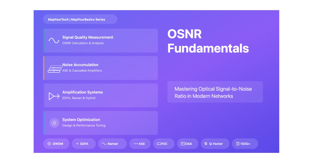
MapYourTech · MapYourBasics Series

OSNR Fundamentals

Optical signal-to-noise ratio from first principles — the physics of ASE, the 58 formula, modulation-format thresholds, and link budgeting you can run yourself.

Introduction

Optical signal-to-noise ratio is the dominant performance parameter in an amplified optical link, because it sets the bit error rate the receiver must work with and the distance a wavelength can travel before regeneration. OSNR is the ratio of optical signal power to optical noise power inside a defined reference bandwidth — conventionally 0.1 nm, about 12.5 GHz at 1550 nm, measured on an optical spectrum analyzer. This guide builds OSNR from the physics of amplified spontaneous emission, derives the planning formula engineers actually use, maps OSNR to modulation-format reach, and gives you four calculators to run link budgets directly. It is written for the engineer who has to answer a concrete question: will this wavelength close over this route, and what is the margin?

Definition: OSNR (dB) = 10·log₁₀(P_signal / P_noise), with P_noise the amplified-spontaneous-emission power integrated over the 0.1 nm reference bandwidth.

1. Fundamentals and Core Concepts

Why OSNR degrades

Every optical amplifier on a route injects amplified spontaneous emission alongside the signal it boosts. That noise never disappears: the next amplifier amplifies both the signal and the ASE that preceded it, then adds its own fresh ASE on top. The dominant mechanisms are:

Amplified spontaneous emission (ASE): When an erbium-doped fiber amplifier (EDFA) amplifies the signal, spontaneous photon emission across the gain bandwidth is amplified with it. ASE accumulates with every amplifier stage and is the primary noise source in long links. The noise figure of each amplifier controls how much it adds.

Cumulative noise accumulation: In multi-span systems with cascaded amplifiers, ASE powers add linearly. Each amplifier contributes more noise, degrading OSNR progressively from transmitter to receiver.

Fiber attenuation: As the signal weakens across a span before reaching the next amplifier, the power feeding that amplifier drops; lower input power into a fixed-NF amplifier yields lower per-span OSNR.

Where OSNR is the binding constraint

Long-haul networks spanning hundreds to thousands of kilometres with many amplifiers
High-rate systems at 100G, 400G and beyond, which need higher OSNR for the same reach
High-order modulation such as 16-QAM and 64-QAM, which are far more sensitive to noise than QPSK
Dense WDM systems where many channels share the amplifier gain budget
Submarine systems with 50 or more amplifiers, where OSNR is the reach-limiting factor

Operational consequences

OSNR sets the receiver bit error rate, and BER falls steeply as OSNR rises: roughly 20 dB OSNR can support a pre-FEC BER near 10^-12 for QPSK, while 15 dB pushes it toward 10^-9. It bounds how far a signal travels before regeneration, and it acts as the quality-of-service metric at the physical layer — degradation there surfaces as packet loss at higher layers. Most design decisions trace back to it: amplifier count, span spacing, modulation choice, and FEC strength.

Takeaway: No amount of receiver DSP recovers OSNR that was never delivered. ASE added in the line is permanent; the only levers are lower-noise amplifiers, shorter spans, distributed gain, or stronger FEC.

2. Mathematical Framework

Core definitions

OSNR definition

OSNR = P_signal / P_noise

OSNR (dB) = P_signal(dBm) − P_noise(dBm)

Where: P_signal is the per-channel optical power and P_noise is the ASE power measured in the reference bandwidth (12.5 GHz / 0.1 nm).

The planning formula (the “58” form)

For a single amplified span where the amplifier exactly compensates the preceding loss, the per-span OSNR is:

Per-span OSNR

OSNR_span (dB) = 58 + P_launch − L_span − NF

Where:

P_launch: per-channel power launched into the span (dBm)
L_span: span loss the amplifier must overcome (dB)
NF: amplifier noise figure (dB), 4–6 dB for a typical EDFA
58: the magnitude of 10·log₁₀(h·ν·Δf) at 193.4 THz over a 12.5 GHz (0.1 nm) reference — note the sign is +58, not −58

For N identical spans, the ASE powers add, so the receiver OSNR drops by 10·log₁₀(N):

Multi-span receiver OSNR

OSNR_RX (dB) = 58 + P_launch − L_span − NF − 10·log₁₀(N)

The amplifier gain G does not appear: OSNR is a ratio, and gain acts equally on signal and noise, so it cancels. This is the same relation the EDFA design literature uses for first-order budgeting.

Practical Example — 400 km link with five EDFA spans.
System: launch 0 dBm/channel, fiber 0.25 dB/km, 80 km spans (5 spans), NF 5 dB.
Span loss L = 0.25 × 80 = 20 dB.
Per-span OSNR = 58 + 0 − 20 − 5 = 33 dB.
Receiver OSNR = 33 − 10·log₁₀(5) = 33 − 7.0 = 26 dB.
A 26 dB receiver OSNR closes QPSK and 8-QAM with margin and supports 16-QAM with FEC. The link is comfortably feasible — the binding constraint at this reach is nonlinear penalty from launch power, not ASE.

Common error: writing per-span OSNR as “P_TX + G − L − NF” produces a near-zero or negative number and wrongly condemns a healthy link. The amplifier gain cancels; the bandwidth constant (+58) is what sets the scale. Always anchor to the 58 form.

OSNR, Q-factor and BER

Q-factor from OSNR

Q_dB = OSNR_dB + 10·log₁₀(B_o / B_e)

Where: B_o is the optical reference bandwidth and B_e the electrical receiver bandwidth.

BER from Q-factor

BER = ½ · erfc(Q / √2)

The Q-factor / BER relationship is the bridge from a physical-layer OSNR number to an error rate: a Q of about 7.0 (16.9 dBQ) corresponds to a pre-FEC BER near 10^-12. Modern coherent links operate at far higher pre-FEC BER and lean on strong FEC to reach an error-free post-FEC floor.

3. Noise Sources, Amplifiers and Modulation

Noise sources

Table 1: Optical-domain noise sources and mitigation
Noise source	Description	Typical impact	Mitigation
ASE	Spontaneous emission in the EDFA gain medium amplified with the signal	Primary source; sets per-span OSNR via NF	Low-NF amplifiers, optimal pump power
Spontaneous Raman scattering	Random scattering in Raman amplifiers from pump-phonon interaction	Distributed along the fiber	Counter-pumping, distributed gain
Receiver thermal noise	Electronic noise in the photodetector and front end	Fixed floor, dominant at low received power	Low-noise detectors
Shot noise	Quantum noise from discrete photon arrivals	Fundamental quantum limit	Cannot be removed, only minimised

Amplifier choice and its OSNR cost

Table 2: Amplifier types and effective noise figure
Amplifier type	Noise figure	OSNR impact	Best use case
EDFA (single stage)	5–6 dB	Baseline	General purpose, cost-effective
EDFA (dual stage)	4–5 dB	Improved	Long-haul
Raman (distributed)	−2 to 0 dB (effective)	Large improvement	Ultra-long-haul, submarine
Hybrid (EDFA + Raman)	2–3 dB	Best	Maximum reach
SOA	6–10 dB	Higher noise	Metro, short reach

The quantum floor on EDFA noise figure is 3 dB — one noise photon per signal photon of gain. Hybrid EDFA+Raman amplification can reach an effective NF below the EDFA-only floor because the distributed Raman gain amplifies the signal before it has fully decayed.

OSNR required by modulation format

Table 3: Representative OSNR thresholds by modulation format
Format	Bits/symbol	Required OSNR	Typical application
NRZ (OOK)	1	15–18 dB	10G systems
DPSK	1	13–15 dB	40G improved sensitivity
QPSK	2	11–15 dB	100G coherent
8-QAM	3	17–20 dB	200G
16-QAM	4	21–25 dB	400G high capacity
64-QAM	6	27–30 dB	Short reach, DCI

Takeaway: Each step up in modulation order buys spectral efficiency at a steep OSNR price — 16-QAM needs roughly 10 dB more than QPSK. The format you can run is whatever the receiver OSNR, minus FEC credit and margin, will support.

4. Effects and Impacts

Bit error rate: As OSNR falls, the receiver separates the signal levels less cleanly and BER rises steeply — a 3 dB OSNR drop can move BER by several orders of magnitude.

System reach: Poor OSNR caps the distance before regeneration; each decibel of improvement extends reach by roughly 10–15 km in typical long-haul systems.

Modulation constraint: Insufficient OSNR forces a lower-order format. A link at 18 dB may be limited to QPSK while 25 dB enables 16-QAM, doubling spectral efficiency.

FEC overhead: Lower OSNR demands stronger FEC, which adds bandwidth overhead and latency. Soft-decision FEC recovers several dB of OSNR penalty at the cost of complexity.

Table 4: OSNR operating bands
OSNR range	Level	Typical BER	System status
> 25 dB	Excellent	< 10^-15	Supports 16-QAM and higher
20–25 dB	Good	10^-12–10^-15	QPSK, 8-QAM with FEC
15–20 dB	Marginal	10^-9–10^-12	Strong FEC, limited reach
< 15 dB	Poor	> 10^-9	Regeneration needed

Capacity follows Shannon: C = B·log₂(1 + SNR), so a 6 dB OSNR reduction roughly halves the theoretical channel capacity. The cascade limit is set directly by the 10·log₁₀(N) penalty — doubling the number of amplifiers costs 3 dB of receiver OSNR, which is the lever the next section's calculators expose.

5. Interactive Calculators

Four calculators built on the same physics: OSNR = 58 + P_launch − L_span − NF − 10·log₁₀(N). Adjust the sliders to see how launch power, noise figure, span loss and amplifier count trade against receiver OSNR and modulation reach. The fifteen-second test: hold everything fixed and double the span count — the receiver OSNR drops by exactly 3 dB.

6. Improvement Techniques

Reduce span length

Shorter spans mean less loss before each amplifier, raising per-span OSNR. Cost is more amplifiers and management overhead. Terrestrial systems favour 80–100 km; submarine systems use 50–60 km.

Low noise figure amplifiers

EDFAs below 4.5 dB NF cut ASE directly — a 1 dB NF improvement is about 1 dB of per-span OSNR. Dual-stage designs with 980 nm forward pumping serve the pre-amplifier and critical stages.

Distributed Raman amplification

Using the transmission fiber as the gain medium gives an effective NF of −2 to 0 dB and can extend reach 30–50%. Cost is high-power pumps (500–1000 mW) and more complex pump management; counter-propagating pumps avoid signal-pump interactions.

Hybrid EDFA + Raman

Combining distributed Raman gain with discrete EDFAs reaches an effective NF of 2–3 dB and the best overall OSNR, at the highest complexity. Reserved for ultra-long-haul and submarine routes beyond 1500 km.

Forward error correction

Hard-decision FEC gives 5–6 dB of coding gain; soft-decision FEC reaches 10–11 dB, letting the link run at a lower OSNR threshold. Overhead is 7–20% and latency rises.

Launch power management

Higher power lifts OSNR linearly until fiber nonlinearities (SPM, XPM, FWM) dominate. Per-channel power of −1 to +2 dBm is the usable window for DWDM.

Table 5: Improvement techniques compared
Technique	OSNR improvement	Cost	Complexity
Shorter spans	2–3 dB/span	High	Low
Low-NF EDFA	1–2 dB/amp	Medium	Low
Raman	3–5 dB effective	High	High
Hybrid EDFA+Raman	5–7 dB	Very high	Very high
Advanced FEC	10–11 dB coding gain	Medium	Medium
Power optimisation	1–3 dB	Low	Low

7. Design Methodology

The design flow is: define requirements, set the required OSNR for the chosen format, build the loss budget, size amplifier spacing, compute end-to-end OSNR with the 58 formula, then verify margin and nonlinear limits. The full DWDM link-design parameter set adds GOSNR, PMD and PDL budgets on top.

Practical Example — 1000 km, 100G QPSK, 80 DWDM channels.
Required OSNR 15 dB; add 3 dB margin → 18 dB target; 7% HD-FEC.
Span loss = 80 × 0.25 + 2 = 22 dB; spans = ceil(1000/80) = 13; NF 5 dB; launch 0 dBm.
Receiver OSNR = 58 + 0 − 22 − 5 − 10·log₁₀(13) = 58 − 22 − 5 − 11.1 = 19.9 dB.
Margin = 19.9 − 18 = 1.9 dB. Feasible but tight — dropping NF to 4 dB or adding Raman lifts the margin above 3 dB and leaves room for aging.

Table 6: Common design pitfalls
Pitfall	Impact	Prevention
Ignoring component losses	2–5 dB underestimate	Include connectors, splices, ROADMs
No system margin	Aging causes failures	Carry 3–6 dB for aging and repairs
Excessive launch power	Nonlinear OSNR penalty	Cap near +2 dBm/channel in DWDM
Ignoring cascaded ASE	Overestimated OSNR	Apply the 10·log₁₀(N) penalty
Ignoring temperature	1–2 dB variation	Test across range, add margin

8. Applications and Case Studies

OSNR targets shift with the deployment. A metro ring with ROADM add/drop (5–8 dB per node) aims above 22 dB; a 500–1500 km long-haul link targets 18–20 dB with low-NF EDFAs and continuous OSNR monitoring; a 5000–10000 km submarine system runs 15–17 dB with hybrid amplification and SD-FEC, plus 2–3 dB of aging margin over a 25-year life.

Practical Example — 400G DCI upgrade over 120 km.
An existing 100G link delivered 22 dB OSNR; 400G 16-QAM needs about 23 dB. Switching to low-NF EDFAs (5.0 → 3.8 dB), lifting launch to +2 dBm, adding Raman pre-amplification, and deploying 20% SD-FEC raised OSNR to 25.5 dB — a 2.5 dB margin above requirement — taking the fiber pair from 10 Tb/s to 40 Tb/s without new fiber.

Practical Example — long-haul OSNR drift.
A 1200 km QPSK link operating at 15.5 dB OSNR drifted 2 dB over three years. Root causes: two EDFA pumps below spec, dirty connectors, one degraded splice. Replacing the pumps recovered 1.2 dB, cleaning connectors 0.5 dB, and a splice repair 0.3 dB — restoring OSNR to 17.5 dB and pre-FEC BER from 10^-9 to 10^-12. The lesson is design-time aging margin plus continuous monitoring.

Table 7: OSNR targets by application
Application	Distance	Data rate	Target OSNR
Metro ring	50–300 km	100G–400G	> 22 dB
Data center interconnect	80–120 km	400G–800G	> 24 dB
Long-haul	500–1500 km	100G–200G	> 18 dB
Ultra-long-haul	1500–3000 km	100G	> 16 dB
Submarine	5000–10000 km	100G–200G	> 15 dB

Main Points

1. OSNR is the dominant physical-layer metric — it sets BER and reach.

2. ASE powers add linearly through cascaded amplifiers; receiver OSNR falls by 10·log₁₀(N).

3. The planning formula is OSNR = 58 + P_launch − L_span − NF − 10·log₁₀(N); gain cancels.

4. Per-span OSNR is set by launch power, span loss and NF — not by amplifier gain.

5. Higher-order modulation needs far more OSNR — 16-QAM about 10 dB above QPSK.

6. Low-NF amplifiers, Raman, shorter spans and FEC are the levers to recover OSNR.

7. Carry 3–6 dB margin for aging, temperature and component drift.

8. Continuous OSNR monitoring catches degradation before it reaches the BER floor.

References

ITU-T, Optical interfaces for multichannel systems with optical amplifiers (G.692), ITU-T Study Group 15.
ITU-T, Optical monitoring for dense wavelength division multiplexing systems (G.697), ITU-T Study Group 15.
ITU-T, Forward error correction for high bit-rate DWDM submarine systems (G.975.1), ITU-T Study Group 15.

Sanjay Yadav, "Optical Network Communications: An Engineer's Perspective" — Bridge the Gap Between Theory and Practice in Optical Networking.

Developed by MapYourTech Team

For educational purposes in Optical Networking Communications Technologies

Note: This guide is based on industry standards, best practices, and real-world implementation experiences. Specific implementations may vary based on equipment vendors, network topology, and regulatory requirements. Always consult with qualified network engineers and follow vendor documentation for actual deployments.

Feedback Welcome: If you have any suggestions, corrections, or improvements to propose, please feel free to write to us at [email protected]

Start with DWDM Fundamentals

871+ Technical Articles

Engineering Knowledge Base

OSNR Fundamentals

OSNR Fundamentals

Introduction