
DWDM Channel Monitoring with OCM and OSA
Optical Channel Monitors versus Optical Spectrum Analyzers — measured parameters, deployment architectures, inline and tap-based monitoring, and integration with network management systems.
1. Introduction
The foundation of optical performance assurance in live DWDM networks
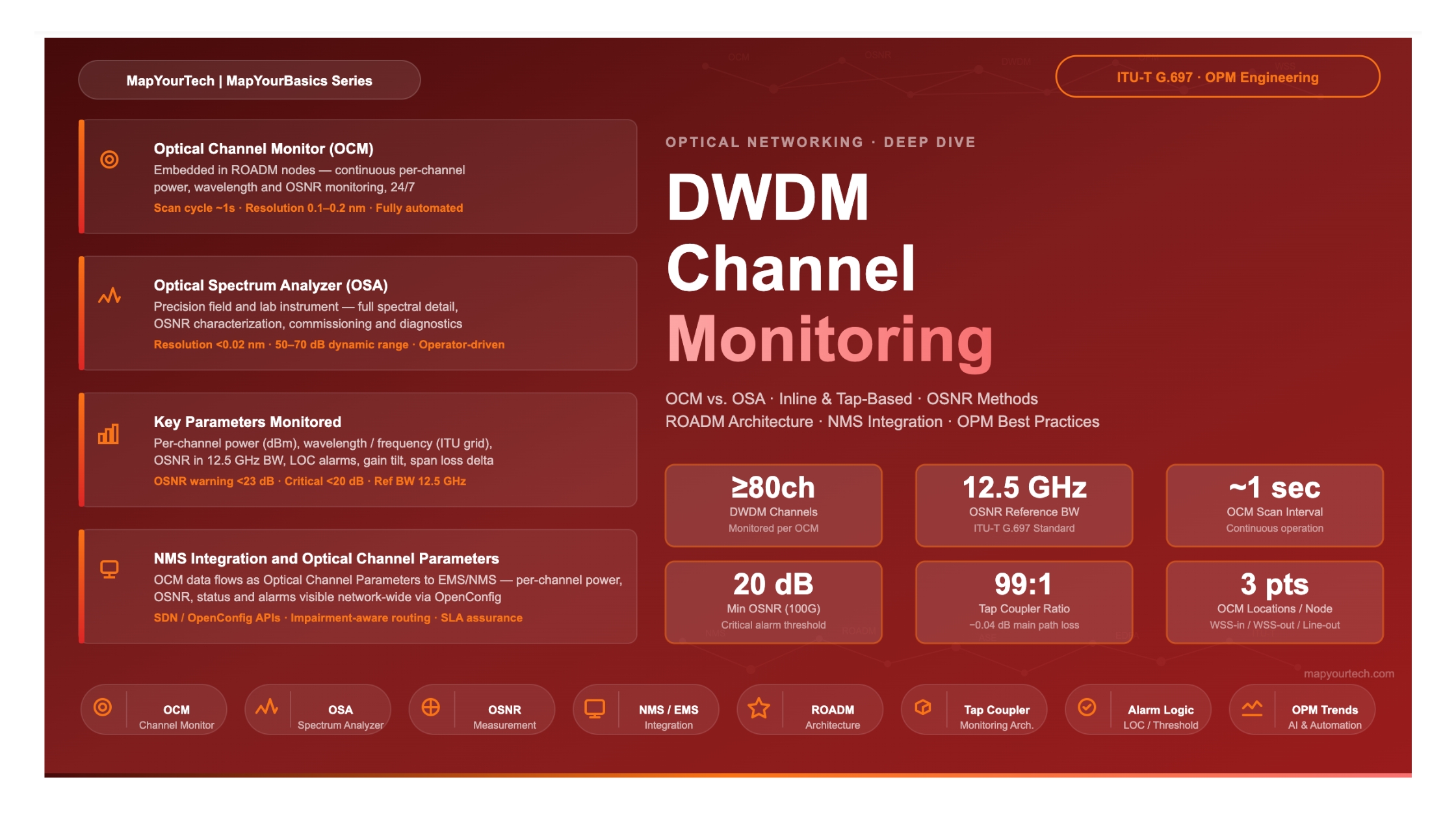
Dense Wavelength Division Multiplexing (DWDM) networks carry enormous volumes of traffic across dozens — and in many modern deployments, up to 96 or more — individual optical channels co-propagating on a single fiber pair. Each of those channels carries its own laser wavelength aligned to the ITU-T frequency grid, its own power level set by the amplifier and attenuation chain, and its own signal quality margin determined by the accumulated noise and impairments along the path. Keeping all of these variables within acceptable bounds, continuously and across an entire network, is the central challenge of optical performance monitoring (OPM).
Two categories of instrument sit at the heart of that challenge: the Optical Channel Monitor (OCM) and the Optical Spectrum Analyzer (OSA). Both observe the optical spectrum, but they differ profoundly in their design intent, placement philosophy, cost, resolution, and the depth of information they can provide. OCMs are purpose-built for continuous, embedded, in-service monitoring within network nodes — they trade raw spectral resolution for speed, compactness, and the ability to run autonomously inside a line card or ROADM. OSAs are precision laboratory and field instruments capable of resolving fine spectral structure, characterising noise floors with high accuracy, and diagnosing problems that an embedded OCM may flag but cannot fully explain.
Understanding both tools — how they work, what they measure, where they are placed, how their data reaches the network management system (NMS), and how they complement each other — is essential knowledge for any engineer responsible for the design, commissioning, or long-term health of a DWDM network. This article provides that comprehensive treatment, grounded in ITU-T and IEEE standards and in the real-world implementation experience captured in deployed system architectures.
2. Why Channel Monitoring Matters
The physical layer consequences of unmonitored DWDM networks
Optical networks are described as high-capacity, but that capacity comes with fragility at the physical layer. A DWDM channel that drifts in power, shifts in wavelength, or accumulates excessive noise does not announce itself loudly — there is no equivalent of a link-down alarm in the electrical sense. Instead, the bit error rate climbs quietly, forward error correction engines work progressively harder until they saturate, and ultimately a traffic-carrying wavelength fails in a way that a pure electrical monitor would observe only as a client-side service disruption.
Optical performance monitoring exists to observe these changes in the optical domain itself, before they cascade into service impact. The parameters that can alter over time include optical power (which decreases due to fiber aging, connector degradation, or component drift), wavelength (which can shift with laser temperature instability or filter drift), OSNR (which degrades as amplifier noise accumulates or span loss increases), and chromatic dispersion and polarization mode dispersion (which become relevant as network topology changes through ROADM reconfiguration).
The consequences of inadequate monitoring are direct: reduced ability to detect sudden faults, inability to perform root cause analysis on gradual degradations, and the use of excessively conservative system margins — essentially over-engineering the network to tolerate problems that a well-monitored system could correct dynamically. OPM addresses all of these, providing the continuous feedback loop that modern self-managed optical networks depend upon.
Figure 1: Major parameters monitored across a DWDM transmission link from transmitter through fiber, amplifiers, network elements, and receiver.
3. Parameters Measured
Optical power, wavelength, OSNR, and beyond
Optical performance monitors, whether they take the form of an embedded OCM or a benchtop OSA, report on a defined set of physical layer parameters. Understanding what each parameter means, why it is measured, and what range of values indicates healthy operation is a prerequisite to using monitoring data effectively.
3.1 Optical Power per Channel
Optical power is the most fundamental monitored quantity. In a WDM system, the power of each individual channel is tracked in units of dBm. The power level of a channel directly determines whether it will be received with sufficient signal quality and, if it is too high, whether it will induce nonlinear crosstalk onto adjacent channels. Amplifiers use per-channel power information to balance gain flatness across the spectrum. An OCM reads per-channel power at each scan cycle — typically every one to two seconds in deployed systems — and compares it against configured target levels to detect loss-of-channel (LOC) events and low-power or high-power alarms.
In a deployed ROADM implementation, the OCM corrects its reading for the known insertion loss between its physical tap location and the monitored port. For example, if an OCM positioned at the WSS line output reads a channel power of Pread and there is an insertion loss of ILtap between that tap and the booster amplifier input, the reported power is Preported = Pread + ILtap. This calibration ensures that the operator sees the actual power at the relevant network port, not simply the raw detector reading.
3.2 Wavelength and Frequency
Wavelength measurement confirms that each channel occupies its assigned ITU-T frequency grid slot. The C-band ITU grid uses 100 GHz channel spacing (approximately 0.8 nm at 1550 nm) as the base, with 50 GHz, 37.5 GHz, and 25 GHz grids used in denser deployments. An OCM can detect whether a channel's centre frequency has drifted outside its assigned slot, which could indicate a failing laser temperature controller or an incorrectly tuned transponder. Wavelength accuracy at the OCM is typically on the order of ±0.1 nm, which is sufficient to distinguish between adjacent 100 GHz channels but may not resolve a 50 GHz misalignment without additional validation by a higher-resolution OSA.
3.3 Optical Signal-to-Noise Ratio (OSNR)
OSNR is the ratio of signal power to amplified spontaneous emission (ASE) noise power, measured within a defined reference bandwidth. The conventional reference bandwidth is 12.5 GHz (approximately 0.1 nm around 1550 nm), which has been the industry standard for expressing OSNR in C-band DWDM systems. OSNR directly determines the signal quality available to the receiver. A reduction in OSNR — caused by increased span loss, amplifier degradation, or a reduction in launched power — translates into a higher bit error rate after the receiver, eventually exceeding the FEC correction threshold.
OSNR = 10 log₁₀ (P_signal / P_ASE)         [dB, in reference bandwidth B_ref = 12.5 GHz]

Where:
  P_signal  = optical signal power per channel   [mW or dBm]
  P_ASE    = ASE noise power in B_ref bandwidth [mW]
  B_ref    = 12.5 GHz  (≈ 0.1 nm at 1550 nm)

Accumulated OSNR across N amplifier spans (equal spans):
  OSNR_total = OSNR_span - 10 log₁₀(N)

For a single EDFA span:
  OSNR_span (dB) ≈ P_in(dBm) - NF(dB) - L_span(dB) - 10 log₁₀(h·ν·B_ref)

  P_in     = per-channel launch power at span input
  NF      = EDFA noise figure (typically 4–6 dB for inline amplifiers)
  L_span  = span insertion loss (fiber + components)
  h·ν     = photon energy at signal wavelength (~8×10⁻²⁰ J at 1550 nm)
Typical minimum OSNR thresholds in deployed systems are approximately 23 dB for normal operation and 20 dB as the warning boundary for 100G coherent channels. Below 20 dB, FEC engines begin to struggle, and below roughly 15–16 dB, uncorrectable errors become frequent. These values are system-dependent and vary with modulation format — a 16-QAM channel requires substantially higher OSNR than a QPSK channel at the same baud rate.
3.4 Additional Parameters
Beyond the core triad of power, wavelength, and OSNR, a complete optical performance monitoring framework tracks chromatic dispersion (CD), polarization mode dispersion (PMD), and polarization dependent loss (PDL). These parameters cannot typically be measured by an OCM — they require more sophisticated analysis available in coherent receiver DSPs or in specialized field test equipment. However, an OCM can indirectly flag the symptoms caused by excessive CD or PMD (anomalous BER behaviour, coherent receiver alarms) that prompt a deeper investigation. The Q-factor, derived from BER, is also tracked as a higher-level indicator integrating the combined effect of all physical impairments.
Optical Power (dBm)
Per-channel received power referenced to 1 mW. Compared against per-channel target (Ptarget) configured in the amplifier control plane. Typical target range: −10 to +3 dBm per channel at node input, depending on span count and amplifier design.
Wavelength / Frequency (nm / THz)
Position of each channel on the ITU-T frequency grid (G.694.1). OCM accuracy typically ±0.1 nm. Detects channel misalignment, laser wavelength drift, and incorrect channel assignment during provisioning or wavelength rerouting.
OSNR (dB in 12.5 GHz)
Signal-to-noise ratio in the reference bandwidth. Out-of-band OSNR measurable by OCM using spectral gaps between channels. In-band OSNR for coherent systems requires DSP estimation or specialized techniques such as polarization-nulling or delay-line interferometry.
Channel Existence (LOC)
Boolean per-channel status: channel present or loss-of-channel. Derived from per-channel power falling below a threshold based on amplifier saturation power, channel count, and channel bandwidth — a critical alarm driving automated protection and fault isolation.
Section Summary
- Optical power, wavelength, and OSNR are the three primary parameters measured by embedded OCMs in operational networks.
- The standard OSNR reference bandwidth is 12.5 GHz (approximately 0.1 nm at 1550 nm), per long-standing industry convention.
- Typical minimum OSNR thresholds for 100G coherent channels are approximately 20 dB for warning and 23 dB for normal operation — exact values depend on modulation format and system design.
- Loss-of-channel (LOC) detection is the most critical real-time alarm, derived from per-channel power thresholds calibrated against amplifier parameters.
4. Optical Channel Monitor — Technology and Operation
Embedded, continuous, real-time optical monitoring inside network nodes
An optical channel monitor is a compact, embedded instrument designed to scan the WDM spectrum continuously inside a network node. Its primary role is operational: it provides the per-channel power and wavelength information that the node's software uses to detect alarms, drive amplifier gain equalization, and report channel status to the network management system. Unlike a laboratory instrument, an OCM must operate autonomously, without user interaction, for years at a time in the field.
4.1 Operating Principle
Commercially deployed OCMs typically employ one of two physical mechanisms: a tunable bandpass filter combined with a single photodetector, or a diffraction grating paired with a detector array. In the tunable filter approach, the filter sweeps across the C-band (or L-band) wavelength range, passing one narrow spectral slice at a time to the photodetector. The detector output as a function of filter centre wavelength produces the power spectrum. The diffraction grating approach disperses all wavelengths simultaneously onto a detector array, enabling snapshot acquisition but requiring careful calibration of the array response.
In a ROADM implementation, the OCM receives a tapped fraction of the signal — typically a −20 dB tap coupler provides about 1% of the signal power to the OCM while 99% continues along the line — or it is accessed through an internal monitor port within the node architecture. The tap is placed at a specific location in the signal path, and the OCM reports are calibrated to reflect power at a defined reference point, such as the booster amplifier input or the WSS line input, by adding the known insertion loss of the tap path.
4.2 Scan Process and Timing
A well-designed OCM scan cycle is arranged to avoid reading power during transients caused by the very gain and attenuation adjustments it is triggering. In practice, the OCM reads the total output power immediately before and after each spectral scan, and discards the scan result if the total power changed by more than a small threshold — typically around 0.5 dB — during the scan window. This ensures that the reported per-channel values reflect a stable operating state rather than a transient. Operations such as gain changes, tilt adjustments, VOA setting changes, and WSS attenuation changes are not performed during an active OCM scan.
The OCM scan interval in deployed systems is typically on the order of one to two seconds — meaning the node controller has fresh per-channel power data available every second or two. This is fast enough to catch sudden channel power excursions (caused by a fiber cut in an adjacent span, a failing amplifier, or a wavelength being added or dropped at a remote ROADM) within a few scan cycles, allowing alarms to be raised and protective actions to be taken within seconds.
Figure 2: Three-port OCM placement within a ROADM node. OCM-1 monitors the WSS line output (booster input), OCM-2 the line output, and OCM-3 the WSS line input. Each reading is calibrated for the tap insertion loss to reflect actual power at the reference port.
4.3 OCM Alarm Generation
The per-channel power data reported by an OCM drives a hierarchy of alarms on the optical channel (OCH) interfaces managed by the node controller. For a channel in normal steady-state operation ("slow zone" in the ROADM state machine), the OCM flags a low-power alarm when per-channel power falls more than 1.0 dB below the configured target and a high-power alarm when it exceeds the target by more than 1.0 dB. Loss-of-channel is declared when the shifted channel power plus the configured attenuation falls more than 3 dB below the target, representing a more severe degradation requiring immediate action.
For newly provisioned channels entering the "fast zone" of the equalization state machine — channels that have just emerged from a loss-of-channel condition — the alarm thresholds reference the OCM at the WSS line output specifically, with a loss-of-channel trigger at 8.5 dB below the target. This asymmetric threshold reflects the operational need to be more lenient during initial channel bring-up while maintaining tight monitoring once the channel has settled.
5. Optical Spectrum Analyzer — Technology and Capabilities
High-resolution spectral characterization for commissioning and diagnostics
An optical spectrum analyzer is a precision measurement instrument that resolves the optical power distribution across wavelength with high accuracy. Where an OCM is optimised for continuous embedded operation with modest spectral resolution, an OSA is designed for the maximum detail needed to characterize a new system during commissioning, diagnose an anomaly that an OCM has flagged but cannot explain, or qualify a fiber span before putting it into service.
5.1 Core Technologies
The most common OSA architecture uses a diffraction grating monochromator — a rotating diffraction grating that sequentially directs different wavelength slices onto a photodetector. The mechanical rotation of the grating allows high wavelength resolution, typically below 0.02 nm for a laboratory-grade instrument, at the cost of acquisition time: a full C-band sweep at maximum resolution may take several seconds. Field instruments with faster sweep speeds sacrifice some resolution for portability and speed. Modern coherent OSAs use a narrowband tunable local oscillator laser and coherent detection to achieve even finer resolution and the ability to measure in-band noise and signal separately — a critical capability for characterizing coherent optical channels where conventional out-of-band noise interpolation is no longer valid.
Optical spectrum analysis in DWDM characterization uses an OSA to measure the power distribution of signals across wavelengths, helping identify channel spacing conformance, power levels, signal integrity, crosstalk, wavelength drift, and amplifier gain flatness issues. OSNR measurement via an OSA applies the conventional technique of interpolating the noise floor between channels, measuring signal power at the channel peak, and computing the ratio referenced to the 12.5 GHz bandwidth. This out-of-band method works well for directly-detected systems but underestimates the in-band OSNR for coherent systems where signal and noise spectra overlap.
5.2 OSNR Characterization in Submarine and Long-Haul Systems
In the context of submarine cable systems and open terrestrial lines, OSNR characterization during assembly and commissioning follows a defined methodology. A representative approach uses ASE noise channels generated by a noise source followed by a wavelength selective switch to fill unused channel slots with a uniform noise floor that simulates actual WDM loading. The OSA then measures OSNR channel by channel across the loaded band. Using ASE noise channels rather than multiple live lasers eliminates polarization-related measurement artefacts that would affect amplifier behaviour and introduces greater measurement robustness. Channel spacing must be wide enough to allow the OSA's optical resolution to access the noise floor between adjacent channels — typically requiring that the OSA resolution bandwidth be narrower than the spectral gap available.
OSNR expressed in a reference bandwidth of 12.5 GHz is the legacy standard measure. In WDM systems where channels are wider than 12.5 GHz — as with 100G and 400G coherent channels at 32 GBaud and above — the actual noise power that impacts system performance must be integrated over the signal bandwidth, not just 12.5 GHz. The term Generalized Signal-to-Noise Ratio (GSNR or GOSNR) extends the OSNR concept to include both ASE noise and nonlinear interference, integrated over the channel bandwidth, providing a more complete picture of system health for modern high-capacity transmission.
GSNR and Modern Coherent Systems
For coherent systems operating at 100G and above, GOSNR (Generalized OSNR) extends the conventional OSNR metric to include nonlinear interference noise across the channel bandwidth. This is particularly relevant for ultra-wideband C+L band deployments and submarine systems where nonlinear effects contribute significantly to system margin. GOSNR expressed at channel baud rate scales simply with the ratio of channel baud rate to reference bandwidth, enabling unified performance predictions across different channel speeds.
5.3 OSA Usage Scenarios in Optical Networks
The typical occasions for deploying an OSA in a live network environment are system commissioning (verifying power levels, OSNR, and spectral shape before turning up traffic), periodic qualification testing (confirming that a link meets its original design specifications after component replacement or fiber rerouting), troubleshooting investigations triggered by OCM alarms that cannot be explained by the node controller alone, and span characterization before adding new wavelengths to a partially loaded system. The OSA is rarely left connected permanently — its role is the in-depth measurement session that OCM data points to but cannot complete alone.
6. OCM vs. OSA — Detailed Comparison
Matching the instrument to the task
OCMs and OSAs are not competing technologies — they are complementary tools with different design points, serving different roles in the optical network lifecycle. The table below compares them across the dimensions most relevant to a network engineer choosing between the two or determining when each is appropriate.
| Parameter | Optical Channel Monitor (OCM) | Optical Spectrum Analyzer (OSA) |
|---|---|---|
| Primary Purpose | Continuous in-service channel monitoring; alarm generation; amplifier control feedback | Detailed spectral characterization; commissioning; deep diagnostics; OSNR measurement |
| Deployment Location | Permanently embedded inside ROADM/OADM node or amplifier shelf; tap-based access | Connected at access points, monitor ports, or fiber taps during measurement sessions |
| Typical Wavelength Resolution | 0.1–0.2 nm (sufficient to distinguish 100 GHz channels; marginal for 50 GHz) | 0.01–0.06 nm (laboratory grade); 0.05–0.1 nm (field portable); sub-pm (coherent OSA) |
| Scan/Acquisition Speed | Full C-band scan in approximately 1 second; continuous operation | Full C-band scan: seconds (portable field) to seconds (lab); real-time display modes available |
| OSNR Measurement | Out-of-band interpolation; suitable for direct-detection systems and coarse estimation for coherent | Out-of-band interpolation (standard); polarization-nulling or coherent detection (in-band, advanced) |
| Dynamic Range | Typically 20–30 dB relative range between channels | Typically 50–70 dB absolute dynamic range |
| Form Factor | Embedded module or small card (line-card integrated); no display | Bench instrument (1–4U rack) or handheld field unit with display |
| Automation | Fully autonomous; results delivered via NMS/EMS APIs | Manual or scripted operation; results displayed or exported; requires operator |
| Measured Parameters | Per-channel power (dBm), centre wavelength, channel existence (LOC), out-of-band OSNR estimate | Full power spectrum, channel peak power, OSNR (various methods), noise floor, spectral shape, crosstalk, gain flatness |
| Cost Model | Per node; integrated into system cost; amortised over node lifetime | Per-unit instrument cost; shared across commissioning and maintenance teams |
| Suitable for Coherent In-Band OSNR | Not directly; requires DSP-based estimation at receiver side | With coherent OSA or polarisation-nulling attachment: yes |
Figure 3: Comparative capability profile — OCM (embedded monitoring) versus OSA (precision measurement). Scores are normalised capability ratings, not absolute values.
6.1 When to Use an OCM
The OCM is the right instrument for any monitoring need that must run continuously, without operator attendance, across a network with many nodes. It provides the real-time visibility needed to detect sudden channel losses, trigger amplifier rebalancing, confirm that newly provisioned wavelengths are at their intended power levels, and feed the NMS with the per-channel health data needed for service assurance dashboards and SLA verification. Every operational ROADM in a commercial DWDM network includes embedded OCM capability as a standard feature because the alternative — relying on end-to-end BER as the only performance indicator — is too slow to catch and localize problems before they affect customers.
6.2 When to Use an OSA
An OSA is the instrument of choice when detailed, high-accuracy spectral information is needed and when the network can be accessed safely with a connected test instrument. Commissioning a new DWDM system requires OSA verification of OSNR across all channels before the system is turned over to live traffic. Troubleshooting a degraded channel that the OCM reports as low-power but with no obvious cause (fiber bend, connector contamination, filter drift) benefits from the OSA's ability to show the full spectral shape of the problem — a narrow notch in the spectrum is visible to an OSA but invisible to an OCM that reports only the integrated channel power. Qualifying a new fiber span, measuring amplifier gain profiles, and characterizing passive component insertion losses all require the precision that only a benchtop or field OSA can provide.
OCM vs. OSA Summary
- OCM: continuous, embedded, autonomous, lower resolution — the operational backbone of a monitored DWDM network.
- OSA: periodic, connected, operator-driven, high resolution — the diagnostic and commissioning tool deployed when depth is needed.
- The two are complementary: OCM flags the problem, OSA diagnoses its root cause.
- For coherent systems, neither standard OCM nor OSA can directly measure in-band OSNR; receiver DSP and specialized coherent test instruments fill that role.
7. Inline and Tap-Based Monitoring Architectures
Where the monitoring instrument connects to the signal path
Connecting an optical monitoring instrument to a live DWDM signal path requires extracting a sample of the signal without significantly disturbing the traffic it carries. Two fundamentally different approaches exist: inline monitoring, where the instrument is placed directly in the signal path and the signal passes through it, and tap-based monitoring, where a coupler diverts a small fraction of the signal power to the monitor while the remainder continues on the main path.
7.1 Tap-Based Monitoring
Tap-based monitoring is the standard approach for all operational OCMs and for OSA access in live networks. A tap coupler — typically with a split ratio of 95:5 or 99:1 — is placed at the monitoring point in the signal path. The 95% or 99% fraction continues to the next component, while the 5% or 1% fraction is routed to the OCM detector or OSA input fibre. A 99:1 (−20 dB tap) coupler reduces the main path signal power by only about 0.04 dB, which is negligible in most system budgets. The tap coupler is a passive, low-insertion-loss, passive element with very high reliability — it introduces no active failure mode into the main signal path.
The limitation of a tap-based approach is that the OCM or OSA receives a scaled-down replica of the signal, not the signal itself. For an OCM, this is perfectly adequate for measuring relative channel powers and wavelengths. For an OSA measuring OSNR, the received noise floor must be above the OSA's noise floor — at very low signal levels (low total input power or when the OSNR itself is already severely degraded), the OCM or OSA may struggle to distinguish signal from noise accurately.
7.2 Inline Monitoring
Inline monitoring, where the monitoring device sits directly in the signal path, is used only for specific applications where a tap is inadequate — for example, optical time-domain reflectometry (OTDR) launches from within a network element for fibre fault location, or certain legacy OPM technologies that required inline access. For the vast majority of modern DWDM networks, tap-based monitoring completely replaces inline approaches because it eliminates the reliability concern of placing an active device in the traffic path and avoids the insertion loss penalty that an inline device would impose on every channel.
7.3 Monitor Port Architecture in ROADM Nodes
Modern ROADM line cards provide dedicated monitor ports — physically distinct fibre connectors that access the internal tap couplers — allowing an external OSA or field instrument to be connected without disturbing live traffic. These ports are typically labelled by the monitoring point they access: for example, a port labelled "MON-PA-OUT" provides access to the signal after the pre-amplifier output tap. The port is passive: connecting or disconnecting an instrument from a monitor port does not affect the main traffic path. This architecture enables field engineers to perform in-service OSA measurements at any node location without any service impact, which is the standard practice for troubleshooting and periodic performance verification.
Figure 4: Tap-based monitoring (standard approach for OCM) versus inline monitoring. Tap couplers divert 1% of signal power with negligible impact on the main path. Inline monitoring places an active device in the traffic path and is reserved for specialised cases.
8. OCM in ROADM Architecture
How embedded OCMs serve the ROADM control plane
In a modern reconfigurable optical add-drop multiplexer (ROADM) node, the OCM is not a standalone accessory — it is a tightly integrated component of the node control architecture, feeding per-channel measurement data into the control software that manages gain, tilt, power equalization, and alarm generation across the entire card.
8.1 OCM Locations Within a ROADM Card
A typical integrated ROADM line card combining a WSS with booster and pre-amplifier EDFAs uses three monitoring points: OCM-1 at the WSS line output (which corresponds to the booster amplifier input), OCM-2 at the line output (after the booster), and OCM-3 at the WSS line input (after the pre-amplifier output). These three points provide visibility into per-channel power at every critical stage of the amplifier and switching chain. Each OCM reading is corrected for the tap insertion loss between its physical location and the defined reference port, ensuring that the power reported to the operator and the NMS reflects the actual power at the labelled port, not the attenuated sample reaching the detector.
8.2 Power Equalization Using OCM Feedback
The primary operational use of OCM data within the ROADM control loop is per-channel power equalization. The target power per channel is calculated based on the amplifier saturation power, the configured power target, any per-channel offset (used to pre-tilt the spectrum to compensate for anticipated Stimulated Raman Scattering effects over long spans), and the channel bandwidth. The WSS attenuator for each channel is adjusted until the OCM-reported power at the WSS line output converges to the target within the configured tolerance. This closed-loop operation runs continuously, correcting for slow drifts in amplifier gain and fiber attenuation.
8.3 Gain and Tilt Control Integration
Beyond per-channel equalization, the OCM data feeds into gain tilt control algorithms. A spectral tilt — where channels at one end of the C-band have systematically higher or lower power than channels at the other end — can arise from amplifier gain tilt (inherent in the erbium gain spectrum) or from Stimulated Raman Scattering, which transfers power from shorter-wavelength channels to longer-wavelength channels over long fiber spans. The OCM, by reporting power for all channels simultaneously in each scan, allows the controller to compute the spectral tilt and apply a counter-tilt through the VOA or WSS attenuation profile.
ROADM OCM Scan Stability Requirement
Operations that change per-channel power — gain adjustments, tilt corrections, VOA changes, and WSS attenuation updates — must not be performed during an active OCM scan. The OCM compares total output power before and after each spectral scan; if the power changed by more than approximately 0.5 dB during the scan window, the results are discarded. This prevents transient power conditions from being reported as false channel power values or triggering spurious alarms.
8.4 Optical Channel Parameters — Optical Channel Parameters
In multi-vendor ROADM networks, the OCM data is made available to the broader network control plane through a structured parameter set known as Optical Channel Parameters (Optical Channel Parameters). For each optical channel traversing a node, the Optical Channel Parameters carries information including channel existence status, per-channel power at the input and output ports, OSNR estimate, accumulated dispersion, accumulated PMD, and PDL. As a channel passes through each ROADM in the network, its Optical Channel Parameters is updated to reflect the current values at that node. The NMS aggregates Optical Channel Parameters data from all nodes to construct an end-to-end view of each channel's health and accumulated impairments.
9. OSNR Measurement Methods
Out-of-band interpolation, polarisation-nulling, and DSP-based estimation
OSNR measurement is one of the most debated topics in optical performance monitoring because the conventional measurement method — valid and widely used for direct-detection systems — has known limitations when applied to coherent DWDM channels. Understanding the available methods, their assumptions, and their limitations is essential for interpreting monitoring data correctly.
9.1 Out-of-Band Interpolation (Conventional Method)
The conventional OSNR measurement method used by OSAs and OCMs reads the optical spectrum across the C-band, identifies the noise floor between channels (where the ASE noise from amplifiers is visible without a signal component), and interpolates this noise floor to the channel frequency. The OSNR is then the ratio of the channel peak power to the interpolated noise level, expressed in the reference bandwidth of 12.5 GHz. This method works well when channels are spaced widely enough (100 GHz or more) to provide clear spectral gaps, when the noise spectrum is relatively flat across the interpolation range, and when no significant signal spectral components leak into the gap region.
For 50 GHz spaced channels at high baud rates (32 Gbaud and above), the spectral gaps between channels narrow significantly and the signal spectrum may extend into the adjacent channel slot, making clean noise floor interpolation difficult or impossible. This is the primary reason why out-of-band OSNR becomes less reliable for modern high-capacity DWDM systems.
9.2 In-Band OSNR for Coherent Systems
For coherent WDM channels, several techniques have been developed to measure in-band OSNR — the noise that is spectrally coincident with the signal and therefore inaccessible to out-of-band interpolation. The polarization-nulling technique exploits the fact that a coherently modulated signal carries a preferred polarization state while ASE noise is unpolarized; by using a polarizer to null the signal polarization component, the residual power is the in-band noise from which the OSNR can be estimated. Delay-line interferometer (DLI) based methods measure the power ratio at the constructive and destructive interference ports of the interferometer: the coherent signal splits differently between the two ports compared to incoherent ASE noise, allowing OSNR computation from the power ratio.
DSP-based OSNR estimation within the coherent receiver is increasingly the preferred approach for in-service monitoring of coherent channels. Pilot symbol and training sequence techniques insert known patterns into the transmitted data stream at known positions and use the SNR estimated from these known patterns to infer the OSNR. Because this approach uses only the receiver DSP and does not require any additional hardware in the network, it is the most practical method for continuous coherent channel OSNR monitoring in operational networks.
Figure 5: Illustrative OSNR vs. distance profile across a multi-span DWDM link — showing OSNR accumulation per span. Values are approximate for a typical 80 km span system with 4 dB EDFA noise figure and −3 dBm per-channel launch power.
9.3 OSNR Calibration and Non-Linearity Effects
In long-haul systems operating at significant launch powers, the apparent OSNR estimated by simple out-of-band or DSP methods can be artificially high because fiber nonlinear distortions — Self-Phase Modulation (SPM), Cross-Phase Modulation (XPM), and Four-Wave Mixing (FWM) — produce noise-like distortions that are indistinguishable from ASE noise in their effect on the receiver but are not captured by the linear OSNR model. An OSNR monitor that ignores nonlinearity will overestimate the true SNR available to the receiver, leading to optimistic margin calculations. This is why the GSNR (Generalized SNR including nonlinear interference) concept has become important for accurate long-haul system design, and why DSP-based OSNR monitoring in coherent receivers increasingly includes calibration for the nonlinear noise contribution estimated from launch power, channel count, and fiber parameters.
10. NMS Integration and the Monitoring Data Chain
From detector to dashboard — how OCM data reaches the operator
The value of an OCM is only realized if its measurements reach the network management system in a timely, structured, and actionable form. The path from OCM detector output to an NMS dashboard involves several layers of processing, formatting, protocol translation, and alarm correlation.
10.1 Element Management System Layer
At the node level, the OCM data is consumed first by the element management layer of the control software running on the ROADM card processor. This layer applies the insertion loss corrections to convert raw OCM readings into calibrated port-referenced power values, evaluates each channel power against the configured Ptarget thresholds, generates per-channel alarms for LOC, low-power, and high-power conditions, and feeds the power data into the gain and tilt equalization algorithms. The element management layer also maintains a scan history, recording maximum and minimum power values over configurable intervals for performance trending.
10.2 Network Management System Layer
The NMS receives performance data and alarms from all network elements, providing a network-wide view of optical channel health. For DWDM and OTN systems, the Transport Domain EMS within the NMS architecture is responsible for collecting OCM-derived data from all ROADM nodes and presenting it in a unified interface. The NMS collects OSNR data from OCMs integrated with the network elements, generates alarms if OSNR falls below the configured threshold (for example, below 20 dB for 100G channels), and triggers automated diagnostic routines to identify and isolate the cause of degradation. Performance management data — including 15-minute and 24-hour interval statistics for key metrics such as OSNR, per-channel power, and span loss — is stored in the NMS performance database for trending analysis.
10.3 Open Interfaces and SDN Integration
Modern NMS platforms expose monitoring data to higher-level orchestration systems through standardised interfaces. OpenConfig data models provide a vendor-neutral schema for configuring and monitoring optical transport network elements, including terminal devices, line amplifiers, and WSS elements. An SDN controller can query OCM-derived performance data via OpenConfig APIs to make traffic engineering decisions informed by current physical layer conditions — for example, avoiding routing new wavelengths through a span where OSNR is already close to its limit, or proactively moving traffic away from a link showing degrading performance trends.
Submarine cable network management systems follow the same architecture with specific extensions for the remote plant — repeaters, branching units, and wet ROADMs — where physical access for manual measurement is impossible. The NMS for a submarine system correlates ROADM optical measurements, span loss values, and repeater performance data to localize faults within a span to within a few kilometres, enabling repair operations to be planned accurately. The integration of OPM data into impairment-aware routing is also a key capability: the NMS can compile an OPM-enabled routing table that includes the current OSNR, accumulated signal distortions, and number of amplifier hops for each candidate path, allowing the path computation element to choose routes that maximize margin.
Figure 6: OCM data processing chain from optical detector through card controller, Optical Channel Parameters, element management system, to NMS dashboards and SDN integration.
11. Practical Examples and Alarm Thresholds
Real-world values and deployment scenarios
The following examples illustrate how the monitoring data described in earlier sections translates into specific alarm conditions and operational responses in a deployed network. All numerical values are drawn from established industry practice and system design principles.
11.1 OSNR Monitoring in a Real-Time Scenario
An optical network operator monitors OSNR across a 1,200 km long-haul DWDM system consisting of 15 spans averaging 80 km each, amplified by 5.5 dB noise figure inline EDFAs. With a per-channel launch power of −3 dBm and a reference bandwidth of 12.5 GHz, the single-span OSNR contribution from each amplifier is approximately 38 dB. After 15 spans of accumulation, the total OSNR is approximately 38 − 10 log₁₀(15) ≈ 38 − 11.8 ≈ 26 dB. The NMS is configured to generate a warning alarm when OSNR falls below 23 dB (allowing approximately 3 dB margin) and a critical alarm below 20 dB. OCMs at the terminal ROADM nodes report OSNR continuously, and the NMS alerts the operations team when any channel OSNR falls below 23 dB, triggering a diagnostic workflow to identify the cause before traffic is impacted.
11.2 Standard Alarm Threshold Reference
| Parameter | Normal Range | Warning Threshold | Critical / LOC Threshold | Action Required |
|---|---|---|---|---|
| OSNR (100G coherent) | > 23 dB | 20–23 dB | < 20 dB | Optimize launch power; check span loss; inspect amplifiers |
| Per-channel power (at node input) | Ptarget ± 0.5 dB | Ptarget − 1.0 dB or + 1.0 dB | Ptarget − 3.0 dB (slow zone LOC) | Amplifier gain check; WSS equalization; fibre inspection |
| Q-factor | > 7 | 6–7 | < 6 | Check FEC overhead; investigate OSNR and CD |
| BER (pre-FEC) | < 10⁻¹² | ~10⁻⁹ | ~10⁻⁶ | FEC saturation risk; investigate impairments |
| Span loss delta | < 0.5 dB from baseline | 0.5–1.5 dB increase | > 1.5 dB increase | Fibre inspection; connector cleaning; OTDR test |
11.3 Channel Commissioning Validation Sequence
When a new wavelength is provisioned across a multi-span DWDM network, the commissioning process uses both OCM and OSA data in a defined sequence. The OSA is first connected at the source ROADM monitor port to verify that the new transponder is on the correct ITU grid frequency, within the specified power level, and that no spectral anomalies are present in the channel profile. After provisioning the cross-connects at each ROADM along the path, the OCM at each intermediate node confirms that the channel is visible at the expected power level as it propagates through the network. At the destination ROADM, a final OSA measurement verifies the end-of-path OSNR against the system design value. If the OSNR margin is adequate and all OCM readings are within target, the channel is declared in service.
11.4 Fault Localization Workflow
When an OSNR degradation alarm is raised by the NMS, the fault isolation workflow proceeds from the end-to-end view to the individual span. The NMS first identifies which channels are degraded and whether the pattern is consistent with a single-point failure (all channels degraded equally, suggesting a single amplifier problem) or a spectrally-selective degradation (only certain wavelengths affected, suggesting filter drift or a partial fiber damage event). OCM data from each node along the affected path is then examined to identify the span where OSNR begins to degrade, locating the problem between two specific nodes. Within that span, an OTDR or correlation-OTDR (C-OTDR) test can then be used to localize the fault to within a specific point on the fibre route.
12. Future Directions in Optical Channel Monitoring
Machine learning, coherent probing, and autonomous optical networks
The trajectory of optical channel monitoring technology points toward deeper integration of artificial intelligence, higher-resolution embedded sensing, and the convergence of monitoring with autonomous network control. Several developments are shaping this direction as of 2025.
DSP-based OPM in coherent receivers continues to advance, with commercial implementations now routinely providing per-channel OSNR, chromatic dispersion, and differential group delay (DGD) estimates from the receiver DSP without any additional hardware. This trend reduces reliance on out-of-band OCM OSNR estimation for coherent channels and moves monitoring intelligence to the endpoints where the most complete signal information is available. Machine learning-based classifiers applied to digital signal analysis can simultaneously identify bit rate, modulation format, OSNR, chromatic dispersion, and DGD — capabilities that go far beyond what any current OCM can provide.
For the OCM itself, photonic integrated circuit (PIC) technology is enabling more compact, lower-cost implementations with improved stability. PIC-based spectrometers eliminate moving parts entirely by using integrated waveguide arrays rather than mechanically-swept gratings, improving reliability and reducing power consumption. Some implementations achieve all-passive spectrometer designs where the spectral demultiplexing is performed by a fixed arrayed waveguide grating (AWG) rather than a tunable element.
At the network level, the vision of closed-loop autonomous optical networks uses OPM data — from OCMs, from coherent receiver DSPs, and from network-level telemetry — as the continuous feedback signal driving AI-based controllers that optimize amplifier settings, channel powers, modulation formats, and routing decisions without manual intervention. This shifts the OPM function from a diagnostic tool that informs human operators to a real-time control input that drives automated network optimization, which represents the most significant transformation in how monitoring data is used.
13. Conclusion
A unified monitoring framework for modern DWDM operations
DWDM channel monitoring with OCMs and OSAs represents a layered, complementary framework that spans the full operational lifecycle of an optical network. The embedded OCM provides the continuous, autonomous, real-time visibility that keeps a network running within its performance envelope — detecting sudden faults, driving amplifier equalization, generating actionable alarms, and feeding the NMS with the per-channel data needed for service assurance. The OSA provides the depth of characterization needed when a problem requires detailed spectral analysis, when a system is being commissioned, or when a performance anomaly cannot be explained by the coarser measurements that an OCM provides.
The three core parameters — optical power, wavelength, and OSNR — form the foundation of what both instruments measure, with OSNR being the most analytically demanding because of its dependence on measurement technique, channel spacing, and the coherent versus direct-detection distinction. The integration of OCM data with the NMS through structured parameter sets like Optical Channel Parameters, and the emerging use of OpenConfig interfaces to expose this data to SDN controllers, positions optical performance monitoring as the physical layer foundation of intelligent, self-managing optical networks.
As coherent receiver DSPs increasingly take over in-band OSNR estimation and machine learning expands what can be inferred from receiver-side analysis, the OCM's role is evolving rather than diminishing — it remains the best source of in-situ per-channel power information at intermediate network nodes, where no receiver DSP is available and where the amplifier control loop depends on fast, reliable channel power data to maintain spectral balance across the entire loaded spectrum.
Glossary
- ASE (Amplified Spontaneous Emission)
- Broadband noise generated by optical amplifiers (particularly EDFAs) that accumulates along a transmission path and degrades OSNR.
- Chromatic Dispersion (CD)
- Pulse broadening caused by different wavelengths propagating at different speeds in optical fiber, measured in ps/(nm·km). Managed through dispersion compensation or DSP-based equalization.
- EDFA (Erbium-Doped Fiber Amplifier)
- Optical amplifier using erbium-doped fiber stimulated by a pump laser to amplify signals in the C-band (approximately 1530–1565 nm). The primary amplification technology for long-haul DWDM systems.
- GSNR / GOSNR (Generalized Signal-to-Noise Ratio)
- Extended OSNR metric that includes nonlinear interference noise in addition to ASE noise, integrated over the channel bandwidth. More accurate than conventional OSNR for high-capacity coherent systems.
- ITU-T G.694.1
- ITU-T Recommendation specifying the frequency grid for DWDM systems, defining channel frequencies at 12.5 GHz, 25 GHz, 37.5 GHz, 50 GHz, and 100 GHz spacing.
- LOC (Loss of Channel)
- Alarm condition raised when a DWDM channel power falls below a threshold defined relative to the amplifier saturation power and channel count, indicating the channel is no longer present or has severely degraded.
- OCM (Optical Channel Monitor)
- Embedded instrument inside a ROADM or amplifier node that measures per-channel optical power and wavelength continuously, feeding data to the node controller and NMS for alarm generation and amplifier control.
- Optical Channel Parameters
- Structured per-channel parameter set in ROADM systems carrying channel power, OSNR, dispersion, PMD, PDL, and status through each node, enabling end-to-end channel health tracking via the NMS.
- OSA (Optical Spectrum Analyzer)
- Precision measurement instrument that resolves the optical power distribution across wavelength with high accuracy, used for commissioning, OSNR characterization, and deep diagnostics.
- OSNR (Optical Signal-to-Noise Ratio)
- Ratio of per-channel signal power to ASE noise power in a reference bandwidth of 12.5 GHz, expressed in dB. The primary performance metric for DWDM channel quality.
- PMD (Polarization Mode Dispersion)
- Pulse spreading caused by birefringence in optical fiber, resulting in differential group delay between the two polarization axes. A limiting factor for high-speed transmission over older fiber plant.
- ROADM (Reconfigurable Optical Add-Drop Multiplexer)
- Network node that can add, drop, or pass through individual DWDM channels under software control, typically using a wavelength selective switch (WSS). The fundamental building block of modern mesh optical networks.
- VOA (Variable Optical Attenuator)
- Adjustable attenuator used to fine-tune per-channel or total power in DWDM systems, enabling power equalization without changing amplifier gain.
- WSS (Wavelength Selective Switch)
- Optical switching component in a ROADM that routes individual wavelengths between ports with programmable per-channel attenuation, enabling both channel routing and power equalization.
References
- ITU-T Recommendation G.694.1 – Spectral grids for WDM applications: DWDM frequency grid.
- ITU-T Recommendation G.697 – Optical monitoring for dense wavelength division multiplexing systems.
- ITU-T Recommendation G.709 – Interfaces for the optical transport network.
- IEEE 802.3bs – 200 Gb/s and 400 Gb/s Ethernet.
- IEC 61280-2-9 – Fibre optic communication subsystem test procedures: Optical signal-to-noise ratio measurement for dense wavelength-division multiplexed systems.
- OpenConfig Working Group – Terminal Device and Optical Line System data models, openconfig.net.
- Sanjay Yadav, "Optical Network Communications: An Engineer's Perspective" – Bridge the Gap Between Theory and Practice in Optical Networking.
Developed by MapYourTech Team
For educational purposes in Optical Networking Communications Technologies
Note: This guide is based on industry standards, best practices, and real-world implementation experiences. Specific implementations may vary based on equipment vendors, network topology, and regulatory requirements. Always consult with qualified network engineers and follow vendor documentation for actual deployments.
Feedback Welcome: If you have any suggestions, corrections, or improvements to propose, please feel free to write to us at [email protected]