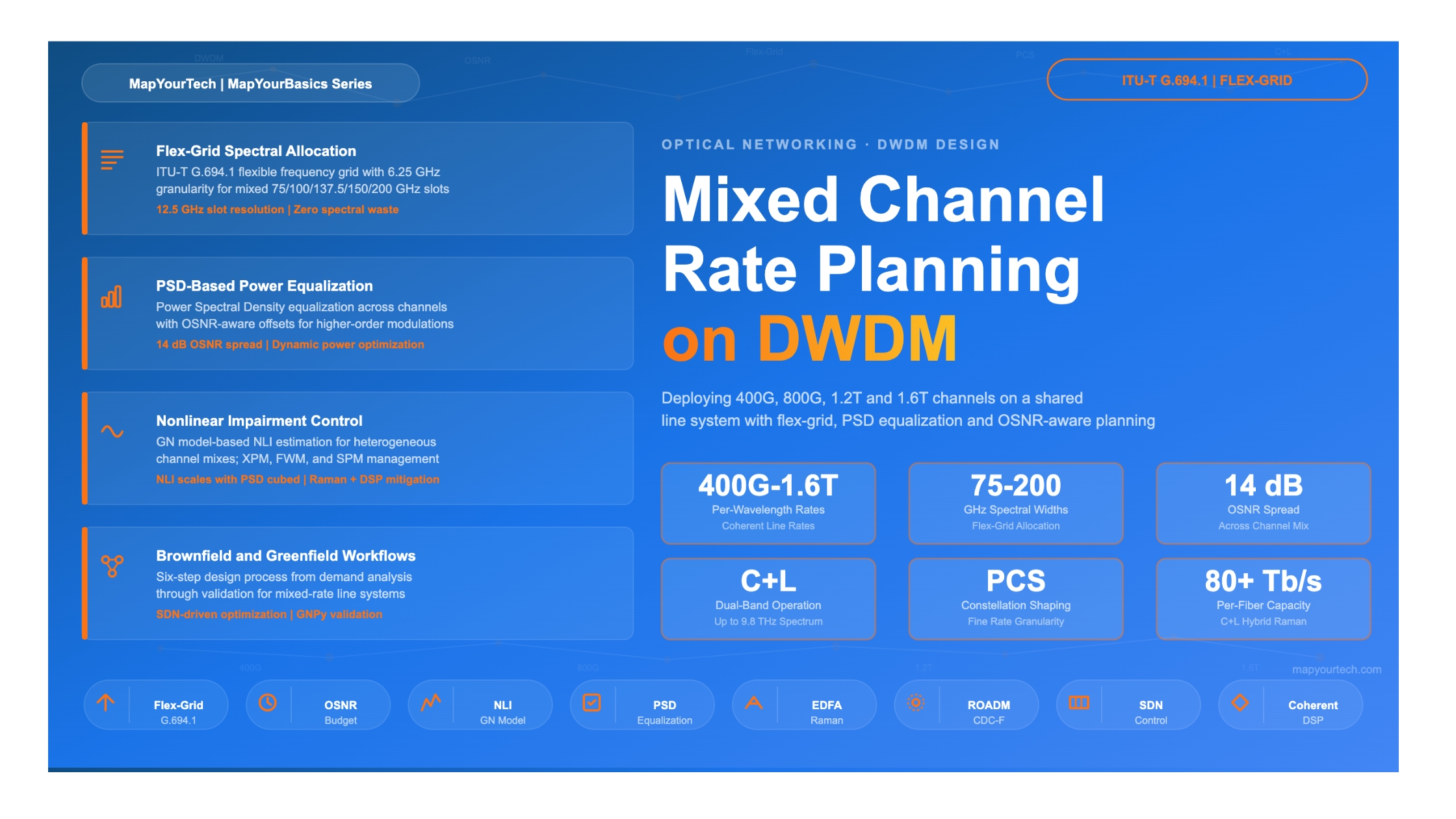

Mixed Channel Rate Planning on DWDM Line Systems
A Design Engineer's Guide to Deploying 400G, 800G, 1.2T and 1.6T Channels on a Shared Optical Line System Using Flex-Grid, Power Equalization and OSNR-Aware Spectrum Planning
Introduction
Modern optical transport networks rarely operate at a single channel rate. A typical backbone or metro fiber route today carries a mix of coherent wavelengths: some provisioned years ago at 100G or 200G, others upgraded to 400G, and the newest slices running at 800G or even 1.2T per wavelength. As operators begin evaluating 1.6T transponders for data-center interconnect and high-capacity metro rings, the challenge of planning all these rates on a single shared line system becomes one of the most complex tasks in optical network engineering.
The move to heterogeneous channel rates on a common fiber is driven by straightforward economics. Ripping out all existing channels to re-deploy at a uniform higher rate is cost-prohibitive and service-disruptive. Instead, network operators follow a pay-as-you-grow approach: new capacity is added at the latest available rate while older channels continue to serve traffic. This results in a spectrum that contains 400G wavelengths occupying 75 GHz slots next to 800G wavelengths in 137.5 GHz slots next to 1.2T or 1.6T wavelengths in 150-200 GHz slots, all sharing the same amplifier chain, the same ROADM cascade, and the same fiber.
This article provides a systematic treatment of mixed-rate channel planning. It addresses the fundamental engineering decisions: how to allocate spectrum using the flexible grid, how to manage per-channel power when OSNR requirements differ by more than 10 dB across the channel mix, how to predict and mitigate nonlinear interference between channels of different bandwidths and modulation formats, and how to validate the design through end-to-end link budgets. The techniques described here apply equally to greenfield deployments designed from day one for multi-rate operation and to brownfield upgrades where new high-rate channels are inserted into partially filled C-band or C+L-band systems.
Fundamentals of Multi-Rate Coherent Transport
2.1 The Flex-Grid Standard and Spectral Slots
The ITU-T G.694.1 recommendation defines a flexible frequency grid where any channel can be centered on a frequency that aligns with a 6.25 GHz grid and occupies a bandwidth that is an integer multiple of 12.5 GHz. This replaces the legacy fixed 50 GHz or 100 GHz grid with a system that can allocate exactly the spectrum each channel needs, and no more. A 400G channel operating at 63 GBd with PCS-16QAM might need only 75 GHz (6 slots of 12.5 GHz), while a 1.6T channel at 200 GBd might occupy 200 GHz (16 slots).
The practical significance of flex-grid in a mixed-rate environment is that it prevents spectral waste. On a fixed 100 GHz grid, a 400G channel that only needs 75 GHz of bandwidth would still consume a full 100 GHz slot, wasting 25% of the allocated spectrum. With dozens of channels across a C-band system, this waste can add up to several terabits per second of lost capacity. The flex-grid approach allows each channel to occupy precisely the bandwidth it requires, with the center frequencies aligned on the 6.25 GHz master grid.
However, flex-grid introduces a spectral fragmentation challenge. When channels of different widths are added and removed over time, gaps can appear in the spectrum that are too small for any new channel but too large to ignore. This fragmentation problem is analogous to disk fragmentation in computing, and it requires careful wavelength assignment algorithms to manage. In mixed-rate systems, the diversity of channel widths (75, 100, 112.5, 125, 137.5, 150, 200 GHz) makes fragmentation more likely than in single-rate systems.
2.2 Modulation Formats, Baud Rates, and Spectral Occupancy
Each coherent channel rate can be realized through multiple combinations of baud rate and modulation format, and the choice directly determines both the required spectral bandwidth and the OSNR sensitivity. A 400G channel, for example, can be transmitted as DP-16QAM at 63 GBd (occupying 75 GHz), or as DP-QPSK at 125 GBd (occupying 150 GHz). The first option is spectrally efficient but requires approximately 20.8 dB of OSNR; the second is spectrally wasteful but survives with about 17.4 dB of OSNR and tolerates far more chromatic dispersion.
The table below summarizes the key operating modes that a design engineer must consider when planning a mixed-rate line system. These values are representative of modern generation-5 and generation-6 coherent DSP platforms.
| Line Rate | Baud Rate (GBd) | Spectral BW (GHz) | Modulation | Bits/Symbol | Required OSNR (dB) | Typical Reach |
|---|---|---|---|---|---|---|
| 400G | 63 | 75 | PCS-16QAM | 3.97 | ~20.8 | Metro/Regional |
| 400G | 88 | 100 | DP-16QAM | 2.84 | ~18.4 | Long-haul |
| 400G | 125 | 150 | DP-QPSK | 2.00 | ~17.4 | Ultra-long-haul |
| 800G | 98 | 112.5 | PCS-16QAM | 5.10 | ~25.4 | DCI/Metro |
| 800G | 138 | 150 | PCS-16QAM | 3.62 | ~23.3 | Regional |
| 1.2T | 138 | 150 | PCS-64QAM | 5.43 | ~31.3 | DCI/Short Metro |
| 1.6T | ~140–200 | 200 | PCS-32QAM | ~5.0 | ~28.0 | DCI/Short Metro |
The spread in required OSNR across the mix is enormous. A 400G DP-QPSK channel at 125 GBd tolerates an OSNR as low as 17.4 dB, while a 1.2T PCS-64QAM channel at 138 GBd demands 31.3 dB. That 14 dB gap means the 1.2T channel requires roughly 25 times more signal-to-noise quality than the 400G channel. Both must coexist on the same amplifier chain, sharing the same total output power. This is the central engineering tension in mixed-rate systems.
2.3 Probabilistic Constellation Shaping and Fine Rate Granularity
Probabilistic Constellation Shaping (PCS) has become a standard feature of modern coherent DSPs. Instead of transmitting all constellation points with equal probability, PCS assigns higher probabilities to low-amplitude symbols and lower probabilities to high-amplitude symbols. This produces a Gaussian-like distribution that approaches the Shannon capacity limit more closely than uniform signaling.
For mixed-rate planning, PCS provides a major advantage: continuous rate tunability. Rather than being locked to discrete rates such as 400G or 600G or 800G, a PCS-capable transponder can deliver any rate between approximately 100G and 1.2T on the same hardware by adjusting the shaping parameters. A transponder initially set to 400G at 75 GHz for a long-haul route can be software-reconfigured to 600G at the same 75 GHz spectral width for a shorter metro route, simply by increasing the constellation order. This fine granularity means that every channel on the line system can be tuned to extract the maximum capacity that the available OSNR on its specific path allows, rather than dropping to the next lower fixed rate.
PCS also reduces the peak-to-average power ratio (PAPR) of the transmitted signal, which lowers sensitivity to fiber nonlinearities. In a mixed-rate system where some channels run at very high spectral efficiency (and hence high PAPR in unshaped operation), PCS provides an additional dB or two of nonlinear tolerance that can make the difference between a channel closing or failing.
2.4 C-Band and C+L-Band Considerations
The conventional C-band spans from approximately 191.35 THz to 196.10 THz, providing roughly 4.8 THz of usable spectrum. At 100 GHz channel spacing, this supports up to 48 channels; at 75 GHz it supports roughly 64 channels. The L-band extends from approximately 186.05 THz to 191.00 THz, adding another approximately 5.0 THz. Together, the C+L band offers approximately 9.8 THz of spectrum.
Mixed-rate planning increasingly involves C+L-band systems because the aggregate capacity of a single C-band simply cannot meet traffic demands on many routes. A C+L-band system with 400G channels at 75 GHz spacing can support roughly 130 wavelengths, delivering approximately 52 Tb/s per fiber. Upgrading some of those channels to 800G increases the per-fiber capacity without adding new fiber. However, C+L operation requires L-band EDFAs (with different gain profiles and higher noise figures than C-band units), Raman amplifiers tuned for the extended band, and wideband ROADMs with L-band-capable Wavelength Selective Switches (WSS).
Spectral Planning and Flex-Grid Allocation
3.1 Bandwidth Assignment Strategy
The first step in planning a mixed-rate line system is to determine how many channels of each rate the spectrum can accommodate. This requires mapping each channel type to its spectral bandwidth, then fitting them into the available C-band (or C+L-band) spectrum like a constrained bin-packing problem.
Consider a concrete example. A C-band system has approximately 4,800 GHz of usable spectrum. The network planner needs to carry a mix of 20 channels at 400G (75 GHz each), 15 channels at 800G (137.5 GHz each), and 4 channels at 1.2T (150 GHz each). The total spectral demand is:
/* Spectral demand calculation */
Spectrum400G  = 20 x 75 GHz  = 1,500 GHz
Spectrum800G  = 15 x 137.5 GHz = 2,062.5 GHz
Spectrum1.2T  =  4 x 150 GHz = 600 GHz
─────────────────────────────────────
Total demand  = 4,162.5 GHz
Available C-band = ~4,800 GHz
Remaining     = 637.5 GHz (room for ~8 more 400G@75GHz or ~4 more 800G@150GHz)
Total capacity = (20 x 400) + (15 x 800) + (4 x 1200) = 24.8 Tb/s
Guard bands between channels of different spectral widths are typically not required in flex-grid systems because the WSS filter shape provides adequate isolation. However, when mixing very wide and very narrow channels, some operators add a 6.25 GHz or 12.5 GHz guard band at the boundaries to account for center-frequency offsets and filter roll-off variations.
3.2 Channel Placement Order and Fragmentation Avoidance
The order in which channels are placed in the spectrum affects long-term fragmentation. A recommended approach is to group channels by spectral width. Place the widest channels (1.6T at 200 GHz, 1.2T at 150 GHz) at one end of the C-band, then the medium channels (800G at 112.5–150 GHz) in the middle, and the narrowest channels (400G at 75–100 GHz) at the other end. This "wide-first" strategy creates contiguous blocks of similar-width channels and leaves any residual fragmentation in the narrow-channel region, where it is easiest to fill with small channels.
The SVG diagram below illustrates an optimized mixed-rate C-band spectrum. Each colored block represents a channel, drawn to proportional spectral width. The frequency axis spans the full C-band from 191.35 THz to 196.10 THz (~4,750 GHz). Observe how wider channels (1.6T, 1.2T) are grouped on the low-frequency side and narrower 400G channels on the high-frequency side, leaving any residual gap in the narrow-channel zone where it can most easily be filled.
An alternative approach used in brownfield systems is "first-fit descending": when a new channel is requested, the planner assigns it to the first available contiguous block that fits, scanning from the lowest frequency upward. If the new channel is wider than any single available gap, the planner may need to defragment the spectrum by reassigning existing channels to new frequencies, a process called spectrum defragmentation or "hitless retuning" if performed without traffic interruption.
The fragmentation comparison above shows the practical difference between the two approaches. In the random/ad-hoc scenario (top bar), channels were provisioned as demand arrived without regard for spectral width grouping. The result is six small gaps scattered across the band, each too narrow to fit even a 400G channel at 75 GHz. Roughly 90 GHz of spectrum is stranded in these fragments. In the wide-first scenario (bottom bar), the same set of channels is reordered so that all free spectrum consolidates into a single contiguous block at the high-frequency end of the band. This block can accommodate any future channel rate, from 400G at 75 GHz to 1.6T at 200 GHz.
When a brownfield system has become fragmented, some modern transponders support "hitless wavelength retuning" where the channel center frequency is shifted without dropping traffic. The transponder briefly transmits on both old and new frequencies, then drops the old one. Combined with an SDN controller that computes an optimal defragmentation plan, this allows the network to recover from fragmentation without planned outages. However, hitless retuning requires that both the transponder and the ROADM WSS support make-before-break operation.
3.2.1 Power Spectral Density View of a Mixed-Rate Channel Plan
Beyond the frequency-domain spectrum map, it is instructive to visualize the relationship between each channel's spectral bandwidth and its required launch power. In a PSD-equalized mixed-rate system, the per-channel power scales directly with bandwidth: a channel occupying 200 GHz receives roughly 4.3 dB more power than a channel occupying 75 GHz, but both have the same power spectral density (-17 dBm/GHz in this example). The chart below shows this proportional relationship using a dual-axis view, with light blue bars representing spectral bandwidth (left axis) and solid colored bars representing launch power (right axis).
3.2.2 Spectral Efficiency Across Channel Rates
Each channel rate achieves a different spectral efficiency (measured in bits/s/Hz), which determines how much data can be packed into a given amount of spectrum. Higher-order modulations and tighter spectral widths deliver greater efficiency, but at the cost of reduced reach and tighter OSNR margins. The chart below compares the spectral efficiency of the common operating modes used in mixed-rate systems.
3.3 Channel Count Comparison Across Grid Strategies
The choice of channel spacing directly impacts aggregate capacity. The table below compares the maximum number of channels and total fiber capacity for a single C-band under different grid configurations.
| Grid Strategy | Channel Rate | Spectral Width (GHz) | Max Channels (C-Band) | Aggregate Capacity (Tb/s) |
|---|---|---|---|---|
| Fixed 100 GHz | 400G | 100 | 48 | 19.2 |
| Flex-Grid 75 GHz | 400G | 75 | 64 | 25.6 |
| Fixed 100 GHz | 800G | 100 | 48 | 38.4 |
| Flex-Grid 137.5 GHz | 800G | 137.5 | 35 | 28.0 |
| Flex-Grid 150 GHz | 1.2T | 150 | 32 | 38.4 |
| Flex-Grid 200 GHz | 1.6T | 200 | 24 | 38.4 |
| Mixed (optimized) | 400G+800G+1.2T | 75/137.5/150 | ~39 | ~24–35 |
The key insight is that spectral efficiency (bits/s/Hz) and total fiber capacity are not the same thing. A system filled with 400G channels at 75 GHz achieves roughly 5.3 bits/s/Hz of spectral efficiency but only 25.6 Tb/s total. A system filled with 800G at 100 GHz (using tighter PCS-16QAM modes) achieves 8.0 bits/s/Hz and 38.4 Tb/s. The mixed-rate system typically falls between these extremes, but offers the operational advantage of matching capacity to demand on each path without over-provisioning.
Power Management and Equalization
4.1 The Power Spectral Density Approach
In a system where all channels have the same spectral width, power management is straightforward: set every channel to the same target launch power. In a mixed-rate system, however, channels occupy different bandwidths, and the correct equalization strategy is based on Power Spectral Density (PSD) rather than absolute per-channel power.
The PSD approach sets the power per unit bandwidth to a constant value across the entire spectrum. A channel occupying 150 GHz of bandwidth receives twice the total power of a channel occupying 75 GHz, because it carries noise and signal over twice the spectral width. This ensures that the OSNR per unit bandwidth remains uniform, which is the physically correct equalization target for the amplifier chain.
/* Power Spectral Density equalization */
Pch(dBm) = PSDtarget(dBm/GHz) + 10 x log10(BWch / 1 GHz)

Where:
  Pch       = total channel launch power (dBm)
  PSDtarget = target power spectral density (dBm per GHz reference)
  BWch      = channel spectral bandwidth (GHz)

Example: PSDtarget = -17 dBm/GHz
  400G @  75 GHz: P = -17 + 10 x log10(75)  = -17 + 18.75 = +1.75 dBm
  800G @ 137.5 GHz: P = -17 + 10 x log10(137.5) = -17 + 21.38 = +4.38 dBm
  1.2T @ 150 GHz: P = -17 + 10 x log10(150)  = -17 + 21.76 = +4.76 dBm
  1.6T @ 200 GHz: P = -17 + 10 x log10(200)  = -17 + 23.01 = +6.01 dBm
4.2 OSNR-Aware Power Offset
PSD equalization is the baseline, but it does not account for the fact that higher-order modulation formats are more sensitive to nonlinear interference. A 1.2T channel running PCS-64QAM at 5.43 bits/symbol is significantly more susceptible to cross-phase modulation (XPM) from neighboring channels than a 400G DP-QPSK channel at 2.0 bits/symbol. To address this, some operators apply a deliberate power offset: reducing the launch power of high-modulation-order channels by 0.5–1.5 dB below PSD-equalized levels, and correspondingly increasing the power of lower-order channels.
This approach sacrifices a small amount of OSNR on the sensitive channels (which they can ill afford) but gains a larger benefit in reduced nonlinear penalty. The optimal offset depends on the specific link: the number of spans, the span loss, the fiber effective area (Aeff), and the total channel loading. System vendors typically provide planning tools that compute the optimal per-channel power for a given mixed-rate fill using Gaussian noise model (GN model) approximations.
4.3 EDFA Gain Equalization Challenges
EDFAs amplify all channels in a band simultaneously, and their gain is not perfectly flat across the C-band. Gain flattening filters (GFFs) reduce gain ripple to typically 1–2 dB peak-to-peak, but some wavelength-dependent variation persists. In a single-rate system, this variation is tolerable because all channels have the same OSNR requirement. In a mixed-rate system, a 1 dB gain ripple that slightly penalizes a 400G QPSK channel (which has 5+ dB of margin) could be fatal for a 1.2T PCS-64QAM channel operating with only 2 dB of margin.
The mitigation strategies include selecting amplifiers with low gain ripple (< 1 dB peak-to-peak), placing the most OSNR-sensitive channels in the gain-peak region of the EDFA (typically around 1550–1555 nm in the C-band), and using per-channel power monitoring with VOAs (Variable Optical Attenuators) at ROADM add ports to fine-tune power levels.
When channels are added or removed in a mixed-rate system, the surviving channels experience transient power excursions as the EDFA's automatic gain control (AGC) adjusts. In a system where some channels have very tight OSNR margins, these transients can cause brief error bursts. Fast AGC (sub-millisecond response) and gain-clamped EDFA designs help minimize this effect.
OSNR Budget Engineering for Mixed-Rate Systems
5.1 End-to-End OSNR Calculation
The OSNR delivered to each channel at the receiver is determined by the accumulation of amplified spontaneous emission (ASE) noise across all spans, plus any nonlinear interference noise (NLI). For a multi-span system with Nspan identical spans, each with span loss Lspan (in dB) compensated by an EDFA with noise figure NF (in dB), the linear OSNR for a channel with launch power Pch can be estimated as:
/* OSNR estimation for multi-span link */
OSNRASE(dB) = Pch - NF - Lspan - 10 x log10(Nspan) - 10 x log10(h x v x Bref)

Where:
  Pch    = per-channel launch power (dBm)
  NF      = amplifier noise figure (dB), typically 5–6 dB for C-band EDFA
  Lspan  = span loss (dB), typically 20–25 dB for 80–100 km spans
  Nspan  = number of amplifier spans
  h       = Planck's constant (6.626 x 10⁻³⁴ J·s)
  v       = optical frequency (~193 THz)
  Bref  = noise reference bandwidth (12.5 GHz = 0.1 nm standard)
The effective or "generalized" OSNR (GOSNR) accounts for nonlinear noise as well, using the relation GOSNR-1 = OSNRASE-1 + OSNRNLI-1. In a fully loaded mixed-rate system, the NLI contribution can reduce the effective OSNR by 1–3 dB compared to the ASE-only figure.
5.2 OSNR Margin Allocation
Each channel needs a minimum OSNR to close (the "required OSNR") plus a system margin to account for aging, temperature variations, fiber splices, connector degradation, and unmodeled impairments. The margin allocation is typically:
| Margin Component | Typical Allocation (dB) | Purpose |
|---|---|---|
| End-of-life fiber aging | 1.0–1.5 | Cable degradation over 15–20 years |
| Connector/splice degradation | 0.5–1.0 | Additional loss from maintenance activities |
| EDFA gain variation | 0.5–1.0 | Wavelength-dependent gain ripple |
| Temperature excursion | 0.3–0.5 | Fiber and amplifier temperature sensitivity |
| Unmodeled penalty | 1.0–2.0 | PDL, PMD, filter penalty, nonlinear penalty |
| Total system margin | 3.0–5.0 | Sum of above components |
For mixed-rate planning, the margin requirement may differ by channel type. A 400G DP-QPSK channel with strong FEC can tolerate 3 dB of margin. A 1.2T PCS-64QAM channel, operating much closer to the Shannon limit, may need 4–5 dB of margin to ensure robustness. The conservative approach is to apply the same margin to all channels; the optimized approach is to apply rate-aware margins based on the modulation format's sensitivity.
Nonlinear Impairment Management
6.1 Cross-Channel Nonlinear Interactions
In a mixed-rate system, the primary nonlinear concern is the interference generated by one channel onto its neighbors. The three dominant effects are Cross-Phase Modulation (XPM), Self-Phase Modulation (SPM), and Four-Wave Mixing (FWM).
XPM is typically the dominant nonlinear impairment in multi-channel systems with dispersion-managed or uncompensated fiber. The XPM penalty on a target channel depends on the power and spectral proximity of all interfering channels. A wide 1.6T channel at 200 GHz occupies a larger spectral footprint and generates more XPM interference on its neighbors than a narrow 400G channel at 75 GHz, simply because it carries more total power. Conversely, the 1.6T channel is also more susceptible to XPM from its neighbors because its higher-order modulation format is more sensitive to phase perturbations.
FWM generates spurious frequency components at positions determined by the frequencies of the interacting channels. In flex-grid systems with non-uniform channel spacing, FWM products are less likely to fall exactly on top of an existing channel than in a fixed-grid system with regular spacing. This is an accidental benefit of mixed-rate planning: the irregular spectral widths naturally break the phase-matching conditions that make FWM most efficient.
6.2 The Gaussian Noise Model for Mixed-Rate Systems
The Gaussian Noise (GN) model treats nonlinear interference as an additive Gaussian noise that accumulates with span count. For a mixed-rate system, the NLI power spectral density experienced by a target channel depends on the power spectral density of all channels in the system, not just neighboring ones. The NLI contribution can be expressed as:
/* Simplified GN model NLI estimation */
GNLI(f) = γ2 x Leff2 x Nspan1+ε x GWDM3(f) x BWDM x asinh(π2|β2|LeffBWDM2)

Where:
  γ         = fiber nonlinear coefficient (typically 1.2–1.3 /W/km for G.652)
  Leff      = effective fiber length per span
  ε         = coherence accumulation factor (0 < ε < 1)
  GWDM     = power spectral density of the WDM signal (W/Hz)
  BWDM     = total occupied bandwidth (Hz)
  β2       = group velocity dispersion parameter
The key takeaway from the GN model is that NLI scales with the cube of PSD. This means that even small increases in per-channel power produce large increases in nonlinear noise. In a mixed-rate system, the optimal launch PSD is a compromise: high enough to maintain adequate OSNR for the most demanding channels (1.2T, 1.6T), but low enough that nonlinear penalties do not erode the OSNR advantage.
6.3 Practical Mitigation Strategies
Run each channel at its optimum launch power, which is the point where the sum of ASE noise and NLI noise is minimized. For typical terrestrial systems, the optimum per-channel power is in the range of -2 to +2 dBm depending on span count and fiber type.
Large effective area fibers (Aeff > 110 μm2, such as G.654.E) reduce the nonlinear coefficient γ and directly lower NLI. For new builds carrying mixed high-rate channels, G.654.E fiber provides 2–3 dB of nonlinear advantage over G.652.D.
Distributed Raman amplification reduces the signal power excursion along each span, lowering the peak power in the fiber and hence the NLI. Hybrid Raman-EDFA systems provide 3–5 dB of OSNR improvement, which directly translates to margin for high-rate channels.
Modern coherent DSPs include digital back-propagation (DBP) or perturbation-based NLC algorithms that partially undo intra-channel SPM. These provide 0.5–1.5 dB of effective OSNR recovery, with the benefit more pronounced for high baud-rate channels.
Design Workflow and Implementation
7.1 Step-by-Step Planning Process
Planning a mixed-rate line system follows a structured workflow that proceeds from demand analysis through spectrum assignment to final validation. The following steps represent industry best practice.
Step 1: Demand Analysis. Determine the number and type of channels required on each route. This includes current channels that must be preserved (brownfield) and new channels being added. For each channel, establish the line rate, modulation format, spectral bandwidth, and OSNR requirement.
Step 2: Route Characterization. Inventory the physical route: span count, span losses, fiber type (G.652.D, G.654.E, G.655, etc.), amplifier types and positions, ROADM nodes and their degree counts, and any inline dispersion compensation modules. Measure or estimate the noise figure of each amplifier and the insertion loss of each ROADM express path.
Step 3: OSNR Budget. Compute the end-to-end OSNR for each channel path, accounting for ASE accumulation, ROADM losses, and NLI. Compare the delivered OSNR against the required OSNR plus system margin. Channels that do not close require either a reduction in line rate (e.g., from 800G to 600G), a change in spectral width (wider bandwidth = lower bits/symbol = lower OSNR requirement), or physical improvements (adding Raman amplification, reducing span loss).
Step 4: Spectrum Assignment. Map each channel onto the flex-grid frequency plan. Apply the wide-first placement strategy. Verify that no spectral conflicts exist and that guard bands (if required by local ROADM equipment constraints) are respected.
Step 5: Power Plan. Compute the per-channel launch power using PSD equalization as a baseline, then apply OSNR-aware offsets. Verify that the total power into each amplifier does not exceed its rated input range and that the per-channel power at each ROADM express port is within the WSS operating range.
Step 6: Validation. Run the complete link budget through the vendor's path computation engine (PCE) or an open-source tool such as GNPy. Verify that every channel meets its OSNR target with the required margin. Identify any channels at risk and iterate on the power plan or spectrum assignment.
Figure 3: Mixed-Rate Line System Design Workflow
7.2 Practical Example: Brownfield 800G Upgrade
Consider a regional network with an existing C-band system carrying 40 channels of 400G at 100 GHz fixed spacing (total: 16 Tb/s). The operator needs to add 12 Tb/s of capacity. The options include: (a) adding 30 more 400G channels, which requires a second line system or C+L upgrade; or (b) converting the system to flex-grid and replacing some 400G channels with 800G channels in the freed spectrum.
Option (b) proceeds as follows. The operator first converts the ROADM to flex-grid operation (if the WSS hardware supports it). Then, the 40 existing 400G channels are re-tuned from 100 GHz spacing to 75 GHz spacing, freeing approximately 40 × 25 GHz = 1,000 GHz of spectrum. This freed spectrum accommodates roughly 7 new 800G channels at 137.5 GHz each (7 × 137.5 = 962.5 GHz). The result is 40 × 400G + 7 × 800G = 16 + 5.6 = 21.6 Tb/s, a 35% capacity increase without adding a single new fiber or amplifier shelf.
The engineering challenge in this scenario is that the 800G channels (at PCS-16QAM, requiring ~23–25 dB OSNR) are sharing the amplifier chain with 400G channels (at DP-16QAM or DP-QPSK, requiring ~17–20 dB OSNR). The power plan must be adjusted using PSD equalization, and the total loading increase (from 40 to 47 channels) may push some amplifiers closer to their output power limits, requiring per-channel power reduction that in turn reduces the OSNR of all channels.
Performance Monitoring and Optimization
8.1 In-Service OSNR and Pre-FEC BER Monitoring
Once a mixed-rate system is deployed, continuous monitoring ensures that each channel maintains adequate performance margin over time. The two most informative metrics are per-channel OSNR (measured by the coherent receiver's DSP or by inline optical channel monitors) and pre-FEC bit error ratio (BER), which directly reflects the total signal degradation from all sources.
Pre-FEC BER thresholds vary by channel rate and FEC type. For oFEC (open FEC) implementations common in 400G and 800G transponders, the pre-FEC BER threshold is typically in the range of 1–2 × 10⁻², corresponding to a net coding gain of 11–13 dB. Channels that approach this threshold lose their post-FEC error-free margin and become vulnerable to burst errors from transient events (amplifier add/drop, power surges, fiber vibration).
8.2 Dynamic Power Optimization
Software-defined networking (SDN) platforms can continuously optimize the power plan of a mixed-rate system. By reading telemetry from each channel's DSP (OSNR, pre-FEC BER, nonlinear phase noise) and from each amplifier (gain, output power, tilt), an SDN controller can adjust per-channel power levels in real time to maximize the minimum margin across all channels. This approach is particularly valuable when channels are added or removed, as each change alters the NLI landscape for all surviving channels.
Technology Comparison and Selection Criteria
9.1 Fixed-Rate vs. Flex-Rate Transponders
Fixed-rate transponders operate at a single line rate (e.g., 400G only) with a predetermined modulation format and baud rate. Flex-rate (or "universal") transponders support multiple line rates on the same hardware, typically covering the range from 100G to 800G or 100G to 1.2T. The choice between them directly impacts mixed-rate planning flexibility.
| Criterion | Fixed-Rate Transponder | Flex-Rate Transponder |
|---|---|---|
| Cost per unit | Lower | 10–20% premium |
| Rate flexibility | Single rate | 100G–1.2T software-selectable |
| Spectral width options | 1–2 modes | Multiple (50–200 GHz) |
| PCS support | Often limited | Full PCS with fine granularity |
| Upgrade path | Requires hardware swap | Software license upgrade |
| Inventory management | Multiple SKUs needed | Single SKU for all rates |
| Best use case | Known, stable demand | Evolving, mixed-rate networks |
For networks that plan to carry a mix of rates from day one, or that expect to upgrade channel rates over time, flex-rate transponders are strongly preferred. The initial cost premium is recovered quickly through reduced inventory costs, simplified sparing, and the ability to right-size each channel's capacity to its route without hardware changes.
9.2 Line System Architecture Options
| Architecture | Max Capacity | Mixed-Rate Support | Amplification | Relative Cost |
|---|---|---|---|---|
| C-band EDFA only | ~25–38 Tb/s | Good | EDFA (NF 5–6 dB) | Lowest |
| C-band Hybrid Raman+EDFA | ~30–45 Tb/s | Excellent | Hybrid (eff. NF 0–3 dB) | Medium |
| C+L-band EDFA | ~50–76 Tb/s | Good | Dual-band EDFA | High |
| C+L-band Hybrid | ~65–90 Tb/s | Excellent | Raman + dual EDFA | Highest |
Future Directions
10.1 Towards 1.6T and 3.2T per Wavelength
As of 2025, 1.6T per wavelength is in field trials at several major cloud providers and tier-1 operators. The OIF (Optical Internetworking Forum) has been working on defining 1.6T ZR and ZR+ standards for data-center interconnect applications, building on the established 400G ZR and 800G ZR frameworks. These standards are expected to freeze in the 2026–2027 timeframe, with volume commercial availability following in 2027–2028.
The move to 1.6T and eventually 3.2T will push mixed-rate systems into tighter operating margins. At these rates, the sensitivity to filtering effects in cascaded ROADMs increases, the nonlinear tolerance decreases, and the required OSNR pushes closer to practical system limits. The industry is responding with wider baud rates (140–200 GBd and beyond), improved FEC codes (with net coding gains approaching 13–14 dB), and advanced nonlinearity mitigation in the DSP.
10.2 AI-Driven Network Optimization
Machine learning algorithms are beginning to be applied to mixed-rate network optimization. By ingesting telemetry data from the coherent DSPs and optical amplifiers, ML models can predict the OSNR margin of each channel as a function of total channel loading, then recommend optimal power settings and spectral assignments in real time. Early deployments have demonstrated 1–2 dB of additional margin recovery compared to static planning, which translates directly into higher achievable line rates or longer reach for the same hardware.
10.3 S+C+L Multi-Band Operation
Looking further ahead, the S-band (1460–1530 nm) is being evaluated as a third transmission band to complement C and L. S+C+L operation would approximately triple the available spectrum compared to C-band alone, potentially supporting fiber capacities exceeding 150 Tb/s. However, S-band amplification technology (based on thulium-doped fiber or semiconductor optical amplifiers) is less mature than C-band or L-band EDFA technology, and the interaction between three bands introduces new nonlinear challenges, particularly stimulated Raman scattering between the S-band and L-band.
Conclusion and References
Mixed-rate channel planning on DWDM line systems is a multi-dimensional optimization problem that spans spectral allocation, power management, OSNR budgeting, and nonlinear interference control. The transition from uniform-rate to heterogeneous-rate operation on shared infrastructure is an economic necessity as network operators adopt 800G and 1.2T transponders alongside their existing 400G base. The key engineering principles are: use the flex-grid standard to eliminate spectral waste; equalize power on a PSD basis with OSNR-aware offsets for sensitive high-rate channels; account for the full nonlinear landscape when computing margins; and continuously monitor and optimize the system in service using SDN-driven telemetry.
As the industry progresses toward 1.6T and 3.2T per wavelength, the challenges of mixed-rate planning will intensify. Tighter OSNR margins, higher baud rates, wider spectral footprints, and increased sensitivity to filtering and nonlinear effects will require ever more sophisticated planning tools, more capable DSPs, and more flexible line-system architectures. The engineering foundations described in this article provide the framework for addressing these challenges systematically.
- Flex-grid (ITU-T G.694.1) is the enabling standard for mixed-rate operation, allowing each channel to occupy only the bandwidth it needs.
- Power equalization in mixed-rate systems should be based on Power Spectral Density (PSD), not absolute per-channel power.
- The OSNR spread across a 400G–1.2T mix can exceed 14 dB, requiring careful margin allocation and OSNR-aware power offsets.
- PCS-capable transponders provide fine rate granularity and improved nonlinear tolerance, making them ideal for mixed-rate environments.
- Continuous in-service optimization through SDN controllers and DSP telemetry can recover 1–2 dB of additional margin.
References
[1] ITU-T Recommendation G.694.1 – Spectral grids for WDM applications: DWDM frequency grid.
[2] ITU-T Recommendation G.698.2 – Amplified multichannel DWDM applications with single channel optical interfaces.
[3] OIF Implementation Agreement – 400ZR: 400G Coherent DWDM for DCI Applications.
[4] IEEE 802.3ct – Physical Layer Specifications for 400 Gb/s over DWDM Systems.
[5] Sanjay Yadav, "Optical Network Communications: An Engineer's Perspective" – Bridge the Gap Between Theory and Practice in Optical Networking.
Developed by MapYourTech Team
For educational purposes in Optical Networking Communications Technologies
Note: This guide is based on industry standards, best practices, and real-world implementation experiences. Specific implementations may vary based on equipment vendors, network topology, and regulatory requirements. Always consult with qualified network engineers and follow vendor documentation for actual deployments.
Feedback Welcome: If you have any suggestions, corrections, or improvements to propose, please feel free to write to us at [email protected]