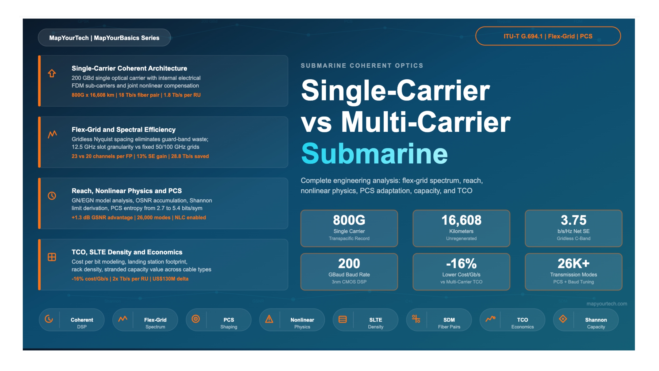
Single-Carrier vs Multi-Carrier Coherent Transmission: Complete Submarine Engineering Analysis
A technical reference covering signal architecture, flex-grid spectrum optimization, reach-capacity trade-offs, nonlinear physics, PCS adaptation, DSP complexity, fiber pair planning, TCO modeling, and interactive decision tools for submarine optical engineers.
1. Introduction: The Carrier Architecture Question
Submarine optical cables form the backbone of global internet connectivity, carrying over 99% of intercontinental data traffic across approximately 600 active cable systems as of 2025. The capacity of these cables has grown dramatically over the past fifteen years, driven primarily by advances in coherent optical technology. The shift from pre-coherent intensity-modulated 10 Gb/s systems to modern coherent transponders delivering 800 Gb/s per wavelength on a single carrier represents an 80-fold per-wavelength capacity increase.
At the core of this evolution lies a fundamental architectural choice: should each high-capacity wavelength be constructed as a single wideband optical carrier, or should the data be distributed across multiple narrower optical sub-carriers combined into a "super-channel"? A third hybrid approach uses a single optical carrier but internally partitions the DSP processing into multiple electrical sub-carriers. Each approach carries different implications for spectral efficiency, reach, nonlinear tolerance, DSP complexity, power consumption, landing station footprint, spectrum sharing, and total cost of ownership (TCO).
This question has taken on renewed significance with the achievement of 800 Gb/s single-carrier transmission across 16,608 km on a transpacific cable in March 2026 — a world record that demonstrated the ability of sixth-generation 3 nm coherent DSPs to deliver ultra-high per-wavelength capacity across the longest submarine routes. Simultaneously, the industry is transitioning from 4–6 fiber pair cables to 12–24+ fiber pair SDM (Space Division Multiplexing) systems, making the per-wavelength spectral efficiency more economically significant than ever.
This article provides a comprehensive engineering analysis of all three carrier architectures, grounded in the physics of long-haul fiber propagation, the mathematics of coherent detection, the economics of submarine cable systems, and recent real-world performance data. All vendor and hardware names have been generalized to maintain neutrality.
2. Signal Architectures Defined
2.1 Architecture A: Single Optical Carrier
In a single-carrier coherent system, the entire data payload of one DWDM wavelength channel is modulated onto a single optical carrier frequency generated by one laser. The transmitter produces one continuous-spectrum signal whose optical bandwidth is determined by the symbol rate and the root-raised-cosine (RRC) pulse shaping roll-off factor. For a sixth-generation DSP operating at 200 GBaud with a typical submarine roll-off of 0.05, the occupied optical bandwidth is Bocc = Rs × (1 + ρ) = 200 × 1.05 = 210 GHz.
The receiver's coherent DSP processes this full-bandwidth signal through a chain of digital equalizers: chromatic dispersion compensation via frequency-domain equalization (FDE), polarization demultiplexing via a 2×2 butterfly equalizer, carrier frequency and phase recovery, and soft-decision FEC decoding. The DSP has full visibility of the entire signal bandwidth, enabling joint optimization and nonlinear compensation across all spectral components.
Single-Carrier Net Rate:
C_net = 2 × R_s × H(X) × (1 - OH_FEC)

Where: 2 = dual polarization, R_s = symbol rate (GBd),
H(X) = PCS entropy (bits/symbol/pol), OH_FEC = FEC overhead

Example: 200 GBd, H(X) = 2.67, FEC = 25%
C_net = 2 × 200 × 2.67 × 0.75 = 800 Gb/s

Spectral occupancy: 200 × 1.05 = 210 GHz
Spectral efficiency: 800 / 210 = 3.81 b/s/Hz
Figure 1: Single-carrier 800G signal. Left: Nyquist-shaped spectrum (~210 GHz) with steep RRC roll-off (ρ=0.05). Right: PCS-64QAM constellation where inner symbols (brighter) are transmitted more frequently, approximating a Gaussian distribution at ~2.7 bits/symbol entropy.
2.2 Architecture B: Multi-Carrier Optical Super-Channel
Multi-carrier transmission distributes the data payload across NSC optically distinct sub-carriers, each generated by a separate laser source or derived from an optical frequency comb. Each sub-carrier is independently modulated at a lower symbol rate and then optically combined into a single "super-channel" that occupies one contiguous block on the flex-grid. Guard bands between optical sub-carriers are required to prevent inter-carrier interference, wasting 5–15% of the available spectrum.
A classic example is a 400G super-channel constructed from four 100G DP-QPSK sub-carriers at ~32 GBaud each, or an 800G super-channel from four 200G DP-16QAM sub-carriers at ~35 GBaud. At the receiver, each sub-carrier is independently detected by a separate coherent receiver with its own local oscillator laser. The DSP for each sub-carrier operates independently and cannot jointly compensate inter-sub-carrier nonlinear interactions.
Figure 2: Multi-carrier 800G super-channel with 4 optical sub-carriers. Red guard bands (~5 GHz) waste ~13% more spectrum vs single-carrier. Each sub-carrier has its own laser and DSP with no joint nonlinear compensation.
2.3 Architecture C: Electrical FDM Within Single Optical Carrier
This hybrid architecture maintains a single optical carrier (one laser, one contiguous spectrum) while internally partitioning the DSP processing into 2, 4, or 8 electrical frequency-division multiplexed (FDM) sub-bands. The key distinction from Architecture B is that all electrical sub-carriers share the same laser and the same optical modulator — the partitioning happens entirely within the digital domain. The optical spectrum appears identical to Architecture A.
Modern sixth-generation DSPs support 1, 2, 4, or 8 internal electrical sub-carriers within the single optical carrier. The March 2026 transpacific 800G world record explicitly used "single-carrier" transmission — meaning Architecture C: one optical carrier with internal electrical sub-carriers, likely 4 or 8, for nonlinearity management across 277 amplifier spans.
Figure 3: Electrical FDM within a single optical carrier. Outer envelope is identical to Figure 1. Dashed lines show DSP-internal partitioning into four 50 GBd electrical sub-bands. Zero optical guard bands. The DSP performs joint NLC across all sub-bands.
4. Flex-Grid Spectrum Allocation Deep Dive
4.1 From Fixed Grid to Flex-Grid: The Evolution
Traditional DWDM systems used a fixed-grid architecture defined by ITU-T G.694.1, with channel spacings of 50 GHz or 100 GHz. These grids were designed for 10G and 40G systems operating at relatively low symbol rates (10–28 GBaud). When coherent technology pushed per-wavelength rates to 100G (at ~32 GBaud) and beyond, the fixed 50 GHz grid became a poor fit: a 32 GBaud signal occupies only ~35 GHz of spectrum within a 50 GHz slot, wasting ~30% of the available bandwidth. Conversely, a 200 GBaud signal requires ~210 GHz and cannot fit into any single 50 GHz or 100 GHz slot.
Flex-grid (also called elastic optical networking) was standardized in the 2012 revision of ITU-T G.694.1. It defines a frequency grid with a 12.5 GHz slot granularity (called a "frequency slot"), where any channel can occupy an integer multiple of 12.5 GHz slots centered on the 6.25 GHz anchor points. This allows channels of different widths to coexist on the same fiber without wasting spectrum.
4.2 Flex-Grid Math for Submarine Systems
Flex-Grid Slot Allocation:

Slot width must be a multiple of 12.5 GHz:
W_slot = n × 12.5 GHz   (n = integer, typically 1-32)

Minimum slot for a signal with baud rate R_s and roll-off ρ:
W_min = R_s × (1 + ρ) + margin

For 200 GBd single carrier, ρ = 0.05:
W_min = 200 × 1.05 + 2 = 212 GHz
Nearest 12.5 GHz multiple: ceil(212/12.5) × 12.5 = 17 × 12.5 = 212.5 GHz

For 95 GBd single carrier (5th-gen DSP), ρ = 0.1:
W_min = 95 × 1.1 + 2 = 106.5 GHz
Nearest 12.5 GHz multiple: ceil(106.5/12.5) × 12.5 = 9 × 12.5 = 112.5 GHz

For 4-SC super-channel at 50 GBd each, ρ = 0.1, guard band = 5 GHz:
W_min = 4 × (50 × 1.1) + 3 × 5 + 2 = 220 + 15 + 2 = 237 GHz
Nearest: ceil(237/12.5) × 12.5 = 19 × 12.5 = 237.5 GHz
4.3 Channel Count Impact: Fixed vs Flex-Grid
| Configuration | Signal BW | Grid Slot | Channels in 4.8 THz C-band | Wasted Spectrum |
|---|---|---|---|---|
| 100G @ 32 GBd on 50 GHz fixed | 35 GHz | 50 GHz | 96 | 31% (15 GHz/ch) |
| 100G @ 32 GBd on flex-grid | 35 GHz | 37.5 GHz | 128 | 7% (2.5 GHz/ch) |
| 400G @ 64 GBd on 75 GHz fixed | 70 GHz | 75 GHz | 64 | 7% |
| 400G @ 64 GBd on flex-grid | 70 GHz | 75 GHz | 64 | 7% |
| 800G SC @ 200 GBd flex-grid | 210 GHz | 212.5 GHz | 22 | 1.2% |
| 800G 4-SC super-ch flex-grid | 237 GHz | 237.5 GHz | 20 | 11.5% (incl. guard) |
| 800G SC @ 200 GBd gridless | 210 GHz | 210 GHz | ~23 | 0% |
4.4 Gridless Architecture in Submarine SLTE
Modern submarine line terminal equipment (SLTE) goes beyond flex-grid to offer a fully gridless architecture. In a gridless system, there are no fixed slot boundaries at all — each wavelength channel occupies exactly the spectrum it needs, and the spacing between adjacent channels is determined solely by the Nyquist criterion (channel spacing equals the baud rate, plus a small margin for laser frequency stability). This eliminates even the 12.5 GHz granularity overhead of flex-grid.
For a 200 GBaud single-carrier system, the minimum Nyquist channel spacing is approximately 200–210 GHz (baud rate plus roll-off and laser margin). In a gridless submarine architecture, channels pack tightly at this spacing, achieving the theoretical maximum channel count for the available bandwidth.
Gridless Channel Count (C-band = 4.8 THz, single-carrier 200 GBd):

N_ch = floor(BW_total / spacing)
N_ch = floor(4800 / 210) = 22 channels

With tighter laser control (spacing = 205 GHz):
N_ch = floor(4800 / 205) = 23 channels

Total fiber pair capacity:
C_FP = 23 × 800 Gb/s = 18.4 Tb/s  (matches the reported 18 Tb/s)

Compared to 4-SC super-channel at same 800G:
N_ch = floor(4800 / 237.5) = 20 channels
C_FP = 20 × 800 = 16.0 Tb/s  (−13% capacity loss vs single-carrier!)

Capacity penalty from using multi-carrier super-channels:
ΔC = 18.4 − 16.0 = 2.4 Tb/s per fiber pair lost
Across 12 fiber pairs: 2.4 × 12 = 28.8 Tb/s stranded capacity
Figure 4: WDM grid comparison. Single-carrier (top) fits 23 channels with Nyquist spacing. Multi-carrier (bottom) fits only 20 due to guard bands. Over 12 fiber pairs, this strands 28.8 Tb/s of capacity.
4.5 Flex-Grid Advantage for Mixed-Rate Submarine Networks
Submarine cables often evolve through multiple technology generations over their 25-year lifetime. A cable deployed in 2025 with 200 GBaud transponders may eventually carry a mix of wavelengths as the SLTE is upgraded: some fiber pairs may carry 800G wavelengths while others carry newer 1.6T wavelengths at different PCS entropies and potentially different baud rates. Flex-grid enables this coexistence by allowing each wavelength to occupy only the spectrum it requires.
WSS-based submarine ROADM branching units support spectrum allocation in 6.25 or 12.5 GHz increments, enabling dynamic redistribution of capacity among landing points as traffic demands change. This is particularly valuable in open cable systems where different consortium members share the same fiber pairs through spectrum sharing agreements.
4.6 Spectral Efficiency Impact of Guard Bands at Scale
| Cable Architecture | FP Count | Ch/FP (SC) | Ch/FP (MC) | Δ Channels | Δ Capacity (Tb/s) | Est. Stranded Value |
|---|---|---|---|---|---|---|
| Regional (700 km) | 6 | 24 @ 1.6T | 21 @ 1.6T | −18 | −28.8 | ~US$14M |
| Transatlantic (6,400 km) | 16 | 23 @ 1.2T | 20 @ 1.2T | −48 | −57.6 | ~US$86M |
| Transpacific (16,600 km) | 12 | 23 @ 800G | 20 @ 800G | −36 | −28.8 | ~US$130M |
| SDM Future (20,000 km) | 24 | 23 @ 800G | 20 @ 800G | −72 | −57.6 | ~US$259M |
5. Spectral Efficiency: Quantitative Analysis
5.1 Defining Spectral Efficiency in Submarine Context
Spectral efficiency (SE) in submarine systems is measured in bits per second per hertz (b/s/Hz) and represents the information throughput per unit of optical bandwidth. It is the single most valuable metric for submarine cable economics because the total usable bandwidth on each fiber pair is fixed by the cable's repeater design and cannot be upgraded after deployment. Every fraction of a b/s/Hz gained translates directly into additional revenue-generating capacity.
Three levels of spectral efficiency are commonly referenced:
1. Raw Modulation SE (per symbol, per polarization):
SE_raw = H(X) bits/symbol/pol
   QPSK: 2.0 | 8QAM: 3.0 | 16QAM: 4.0 | 32QAM: 5.0 | 64QAM: 6.0

2. Net Channel SE (including FEC and Nyquist overhead):
SE_ch = C_net / BW_occupied (b/s/Hz per channel)

3. System SE (including channel spacing, guard bands, edge effects):
SE_sys = C_FP / BW_total (b/s/Hz for entire fiber pair)

Example for 800G single-carrier over 16,608 km:
SE_raw = 2.67 bits/sym/pol (PCS-64QAM shaped down)
SE_ch = 800 / 210 = 3.81 b/s/Hz
SE_sys = 18,000 / 4,800 = 3.75 b/s/Hz
5.2 Shannon Limit and Gap to Capacity
The Shannon capacity formula, adapted for submarine systems with both linear (ASE) and nonlinear noise, provides the theoretical maximum achievable SE for a given signal-to-noise ratio:
Shannon Capacity (per polarization):
C = log2(1 + GSNR) bits/symbol

Where GSNR is the Generalized SNR including both ASE and NLI noise:
GSNR = P_signal / (P_ASE + P_NLI)

Practical capacity with implementation penalty η (dB):
C_practical = log2(1 + GSNR/η) × Loss_signaling

Typical: η = 1.5–2.5 dB, signaling loss = 0.95 (5% OTN overhead)

For dual-polarization over bandwidth BW:
C_total = 2 × BW × log2(1 + GSNR/η) × SO × Loss_sig

Where SO = spectral occupancy = channel BW / channel spacing (≤ 1)
5.3 SE Comparison Across Architectures at Three Distances
| Metric | SC (700 km) | MC (700 km) | SC (6,400 km) | MC (6,400 km) | SC (16,600 km) | MC (16,600 km) |
|---|---|---|---|---|---|---|
| Net Rate/ch | 1,600 Gb/s | 1,600 Gb/s | 1,200 Gb/s | 1,200 Gb/s | 800 Gb/s | 800 Gb/s |
| BW per ch | 185 GHz | 215 GHz | 210 GHz | 238 GHz | 210 GHz | 238 GHz |
| SE (ch) | 8.65 | 7.44 | 5.71 | 5.04 | 3.81 | 3.36 |
| Ch in 4.8 THz | 25 | 22 | 23 | 20 | 23 | 20 |
| FP Capacity | 40.0 Tb/s | 35.2 Tb/s | 27.6 Tb/s | 24.0 Tb/s | 18.4 Tb/s | 16.0 Tb/s |
| SE penalty | — | −12% | — | −13% | — | −13% |
6. Reach Analysis: OSNR, Shannon & GN Model
6.1 Linear OSNR Accumulation
In a chain of N optically amplified spans, the OSNR degrades with each amplifier due to accumulated ASE noise. The end-of-line OSNR for a system with identical spans is:
Linear OSNR (dB):
OSNR = P_launch + 58 − L_span − NF − 10·log10(N_spans)

Where:
  P_launch = per-channel launch power (dBm)
  58 = −10·log(h·f·B_ref) for B_ref = 12.5 GHz at 193.4 THz
  L_span = span loss (dB) = fiber_loss × span_length
  NF = amplifier noise figure (dB)
  N_spans = number of amplified spans

Worked Example — Transpacific (16,608 km):
  Span length: 60 km, Fiber loss: 0.20 dB/km, Span loss: 12 dB
  NF: 5.0 dB, P_launch: −2 dBm
  N_spans: ceil(16608/60) = 277

OSNR = −2 + 58 − 12 − 5.0 − 10·log(277)
OSNR = −2 + 58 − 12 − 5.0 − 24.4 = 14.6 dB

Worked Example — North Sea (700 km):
  N_spans: ceil(700/60) = 12
OSNR = 0 + 58 − 12 − 5.0 − 10·log(12)
OSNR = 0 + 58 − 12 − 5.0 − 10.8 = 30.2 dB
6.2 Nonlinear Shannon Limit
In real submarine systems, increasing launch power to improve OSNR eventually backfires: fiber nonlinearities generate additional noise (NLI) that scales as Pch3. The optimal launch power balances ASE and NLI, creating a maximum achievable GSNR — the nonlinear Shannon limit:
Optimal launch power and max GSNR:

GSNR = P / (P_ASE + η_NL × P3)

Taking derivative, optimal P_opt occurs at:
P_opt = (P_ASE / (2 × η_NL))1/3

At P_opt, the GSNR_max is:
GSNR_max = (2/3) × P_opt / P_ASE

At this point, NLI contributes exactly half the noise of ASE.
The maximum SE is therefore bounded by:
SE_max = 2 × log2(1 + GSNR_max/η) b/s/Hz (dual-pol)
6.3 How Carrier Architecture Affects Reach
The carrier architecture influences the nonlinear coefficient ηNL through two mechanisms: the intrachannel NLI (which depends on signal bandwidth) and the interchannel NLI (which depends on channel spacing and WDM loading). For a single carrier at 200 GBaud occupying ~210 GHz, the intrachannel NLI is marginally higher than for a narrower carrier, but the DSP's ability to apply digital back-propagation (DBP) or perturbation-based nonlinear compensation can recover 0.5–1.5 dB of this penalty.
For multi-carrier super-channels, the individual sub-carriers experience lower intrachannel NLI (each is narrower), but the inter-sub-carrier XPM cannot be compensated since each sub-carrier's DSP operates independently. The net effect varies with distance: at short distances with abundant OSNR, the nonlinear difference is small; at ultra-long distances near the Shannon limit, every fraction of a dB matters, and the single-carrier DSP's ability to perform joint NLC becomes a meaningful advantage.
| Distance | Est. OSNR (linear) | SC GSNR (with NLC) | MC GSNR (no cross-SC NLC) | SC Advantage | SE Impact |
|---|---|---|---|---|---|
| 700 km | ~30 dB | ~25 dB | ~24.5 dB | +0.5 dB | ~2% more capacity |
| 3,000 km | ~22 dB | ~18 dB | ~17.2 dB | +0.8 dB | ~5% more capacity |
| 6,400 km | ~19 dB | ~15.5 dB | ~14.5 dB | +1.0 dB | ~7% more capacity |
| 10,000 km | ~17 dB | ~14 dB | ~12.8 dB | +1.2 dB | ~9% more capacity |
| 16,600 km | ~14.6 dB | ~12.5 dB | ~11.2 dB | +1.3 dB | ~11% more capacity |
7. Nonlinear Propagation Physics: SPM, XPM, FWM
7.1 The Three Nonlinear Enemies
In submarine optical fiber, three primary nonlinear effects degrade signal quality over ultra-long distances: Self-Phase Modulation (SPM), Cross-Phase Modulation (XPM), and Four-Wave Mixing (FWM). Their combined impact is captured by the nonlinear interference (NLI) noise term in the Gaussian Noise model. Understanding how each effect interacts with carrier architecture is essential for making the right design choice.
Self-Phase Modulation (SPM) occurs when a signal's own intensity modulates the fiber's refractive index, inducing a nonlinear phase shift proportional to the signal power. The phase shift accumulates over each amplified span: ΔφNL = γ × Pin × Leff, where γ is the fiber nonlinear coefficient (~1.3 W-1km-1 for submarine fiber with Aeff ~110 μm2). SPM causes spectral broadening and constellation distortion, and is the dominant intrachannel nonlinearity.
Cross-Phase Modulation (XPM) occurs in multi-channel WDM systems when the intensity fluctuations of one wavelength induce phase shifts on neighboring wavelengths. XPM is an interchannel effect and scales with the number and proximity of WDM neighbors. In highly dispersive submarine fiber (D ~ +18 ps/nm/km), the walk-off between channels due to chromatic dispersion partially decorrelates XPM, reducing its impact compared to low-dispersion fiber.
Four-Wave Mixing (FWM) generates parasitic optical frequencies when three wavelengths interact in the fiber. FWM efficiency depends strongly on channel spacing and local dispersion. In modern uncompensated submarine cables with high local dispersion, FWM is significantly suppressed compared to the pre-coherent era when dispersion-managed fibers were used.
7.2 How Carrier Architecture Interacts with Nonlinearities
| Nonlinear Effect | Single Carrier (A/C) | Multi-Carrier Optical (B) | Net Advantage |
|---|---|---|---|
| SPM (intrachannel) | Higher per-carrier SPM due to wider bandwidth. However, the DSP has full visibility and can apply digital back-propagation (DBP) or perturbation-based NLC to partially undo deterministic SPM. | Lower per-sub-carrier SPM (narrower bandwidth each). But each sub-carrier's DSP can only compensate its own SPM — no cross-SC SPM compensation. | SC with NLC wins by ~0.5–1.0 dB |
| XPM (interchannel) | XPM from adjacent WDM channels affects the full carrier bandwidth. DSP nonlinear equalizers can partially mitigate intra-signal XPM using multi-dimensional constellation shaping. | XPM occurs both between optical sub-carriers within the super-channel AND from adjacent WDM channels. Inter-sub-carrier XPM cannot be compensated since DSPs are independent. | SC with joint processing wins |
| FWM (interchannel products) | FWM products from adjacent WDM channels fall within the carrier bandwidth. High local dispersion in submarine fiber suppresses most FWM. | Additional FWM products generated between closely-spaced optical sub-carriers within the super-channel. These fall directly on top of signal frequencies. | SC avoids intra-SC FWM entirely |
Nonlinear Phase Shift Accumulation (per span):

φNL = γ × Pch × Leff

Where L_eff = (1 - e^(-αL)) / α
For 60 km span, α = 0.046 /km (0.20 dB/km):
Leff = (1 - e^(-0.046 × 60)) / 0.046 = ~19.5 km

Total accumulated NL phase over N spans:
φtotal = N × γ × Pch × Leff

For transpacific (277 spans, P_ch = -2 dBm = 0.63 mW):
φtotal = 277 × 1.3 × 0.00063 × 19.5 = ~4.4 radians

This represents massive accumulated nonlinear distortion.
At this level, DSP nonlinear compensation becomes essential,
and single-carrier's ability to perform joint NLC across the
full 200 GBd bandwidth is a meaningful performance lever.
7.3 The Role of High Local Dispersion
Modern submarine cables use pure silica core (P-type) fiber with high local dispersion of +18 to +20 ps/nm/km and large effective area of 100–120 μm2. This fiber design was specifically chosen for coherent-era systems because high dispersion reduces the nonlinear interaction time between neighboring channels (faster walk-off), and large effective area reduces the optical intensity (I = P/Aeff) for a given launch power, directly lowering the nonlinear coefficient.
In highly dispersive fiber, the advantage of splitting into many narrow sub-carriers is smaller than it would be in low-dispersion or dispersion-managed fiber. The dispersion itself acts as a natural nonlinearity suppressant, reducing the marginal benefit of multi-carrier architectures for nonlinear tolerance. This is one reason why single-carrier transmission has become dominant in modern submarine systems — the fiber design has shifted the nonlinear trade-off in favor of wider single carriers with joint DSP processing.
8. Probabilistic Constellation Shaping: Distance Adaptation Engine
8.1 How PCS Approaches the Shannon Limit
Probabilistic constellation shaping (PCS) has become the standard technique for approaching the Shannon capacity limit in submarine coherent systems. The fundamental insight is that the capacity-achieving input distribution for an AWGN channel is Gaussian — not the uniform distribution used by conventional QAM modulation. PCS modifies the symbol probability distribution to approximate this Gaussian shape, transmitting inner (low-amplitude) constellation points more frequently than outer (high-amplitude) points.
For a dual-polarization system using PCS based on a 2m-QAM grid (typically 64-QAM with m=6), the WDM channel information rate is: 2 × BaudRate × (H(X) - m(1 - Rc)) bits/s, where H(X) is the source entropy per polarization and Rc is the FEC coding rate. By varying the PCS entropy H(X) and the FEC code rate Rc, the transponder can continuously tune its operating point along the Shannon capacity curve.
PCS Information Rate (dual-polarization):
C = 2 × Rs × (H(X) - m × (1 - Rc))

Where:
  R_s = symbol rate (GBd)
  H(X) = source entropy (bits/symbol/pol), tunable
  m = QAM grid order (6 for 64-QAM)
  R_c = FEC code rate

For submarine PCS-64QAM at different distances:
  700 km:   H(X) ≈ 5.4  → near full 64-QAM entropy (max = 6.0)
  6,400 km: H(X) ≈ 4.0  → equivalent to 16-QAM performance
  16,600 km: H(X) ≈ 2.7 → shaped down to near-QPSK level

The PCS engine continuously selects the optimal H(X) for
the measured GSNR on each wavelength, approaching the
Shannon limit with ~1.5-2.5 dB implementation penalty.
8.2 The 26,000-Mode Transmission Space
Sixth-generation coherent DSPs operating at up to 200 GBaud combine three independently adjustable parameters to create an extraordinarily fine-grained adaptation space: baud rate (adjustable from 67 to 200 GBaud in fine increments), PCS entropy (continuously tunable from ~1.5 to ~6.0 bits/symbol/polarization), and FEC code rate (multiple SD-FEC options with different overhead levels). The combination of these three axes produces over 26,000 distinct transmission modes.
This granularity means the transponder can extract the absolute maximum capacity from every wavelength slot on every fiber pair, accounting for the specific OSNR conditions, nonlinear noise profile, and spectral position of each channel. Two adjacent wavelengths on the same fiber pair may operate at slightly different modes if their spectral positions experience different EDFA gain profiles or nonlinear penalties.
8.3 Automated Mode Selection
With 26,000 possible modes per wavelength and 23 wavelengths per fiber pair across 12–24 fiber pairs, manual optimization of the channel plan is impractical. Modern SLTE platforms include automated deployment optimization software that performs the following sequence: it probes each wavelength slot with test signals, measures the delivered GSNR including both linear and nonlinear noise contributions, selects the optimal baud rate, PCS entropy, and FEC combination that maximizes the net information rate for each slot, provisions all wavelengths simultaneously, and verifies error-free operation end-to-end.
What previously required weeks of manual engineering by experienced submarine line engineers now completes in approximately two hours. This automation capability is particularly valuable as cable systems scale to 18–24 fiber pairs, where manual optimization would be prohibitively time-consuming and would leave capacity on the table due to human inability to jointly optimize across thousands of interdependent parameters.
9. DSP Architecture, Complexity and Power
9.1 The Silicon Evolution: 7nm to 5nm to 3nm
The coherent DSP is the computational engine of the transponder, performing all modulation, demodulation, equalization, and error correction functions. The progression of CMOS fabrication nodes has been the primary enabler of higher baud rates, more complex algorithms, and lower power consumption:
| DSP Generation | CMOS Node | Max Baud | Max Wavelength | Submarine Max (Trans-Pac) | Power/Bit (Relative) |
|---|---|---|---|---|---|
| 4th Generation | 16nm / 7nm | ~64 GBd | 400G | 200–300G | 4.0× |
| 5th Generation | 7nm / 5nm | ~95 GBd | 800G | 400G | 2.0× |
| 6th Generation | 3nm | 200 GBd | 1.6T | 800G–1.1T | 1.0× |
The leap from 5nm to 3nm was particularly significant for submarine applications. By skipping the 5nm node entirely, the latest generation achieved a 2× increase in baud rate (95 to 200 GBd), which directly translates to double the single-carrier bandwidth and double the per-wavelength capacity. The 3nm process provides 1.6× logic density improvement and 30–35% power reduction at the transistor level, enabling the integration of advanced algorithms (multi-dimensional constellation shaping, nonlinear compensation, edgeless clock recovery) that would not fit within the power and area budget of a 5nm design.
9.2 Chromatic Dispersion Compensation: The Largest DSP Block
Chromatic dispersion (CD) compensation represents the single largest computational burden in a submarine coherent DSP. For a transpacific link at 16,608 km with fiber dispersion of +17 ps/nm/km, the accumulated dispersion exceeds 282,000 ps/nm. The DSP must apply a frequency-domain equalizer (FDE) whose computational complexity scales with both the accumulated dispersion and the square of the signal bandwidth.
FDE Tap Count vs. Carrier Architecture:

Ntaps ∝ |β2| × L × BWsignal2

Pure single-carrier at 200 GBd:
Ntaps ≈ ~28,800 taps (single massive FDE)

Electrical FDM with 4 sub-carriers at 50 GBd each:
Ntaps/SC ≈ ~1,800 taps each
Ntotal = 4 × 1,800 = 7,200 taps (4× reduction)

Electrical FDM with 8 sub-carriers at 25 GBd each:
Ntaps/SC ≈ ~450 taps each
Ntotal = 8 × 450 = 3,600 taps (8× reduction)

This is a primary reason sixth-generation DSPs use electrical
FDM internally: it dramatically reduces CD compensation
gate count, freeing silicon area for NLC and PCS algorithms.
9.3 Carrier Phase Recovery at 200 GBaud
Carrier phase estimation (CPE) tracks the random phase wandering of transmitter and local oscillator lasers. At 200 GBaud, the CPE must make decisions at a rate of 200 billion symbols per second — an extraordinarily demanding requirement on algorithm convergence speed. With electrical FDM sub-carriers, each sub-carrier operates at a lower symbol rate (e.g., 25 GBd for 8 sub-carriers), giving the CPE algorithm 8× more processing time per symbol to converge. This is particularly beneficial when using low-entropy PCS constellations on ultra-long submarine links, where constellation points are dense and phase noise tolerance is tight.
9.4 Multi-Dimensional Constellation Shaping
Beyond per-symbol PCS, sixth-generation DSPs implement multi-dimensional constellation shaping that operates across multiple electrical sub-carriers simultaneously. These shaping techniques encode information jointly across the in-phase and quadrature components of multiple sub-carriers and both polarizations, creating coding gains that are not achievable with per-sub-carrier or per-symbol shaping alone. This capability is specifically designed for submarine links where legacy cable characteristics (compensated or partially compensated dispersion maps) require specialized modulation designs.
10. Fiber Pair Capacity Planning
10.1 C-Band vs C+L Band Capacity
The usable optical bandwidth in a submarine cable is determined by the repeater amplifier design. Conventional C-band EDFAs provide approximately 4.0–4.8 THz of usable bandwidth (1530–1565 nm). C+L band systems, which are now being deployed in some newer cables, extend the amplification bandwidth to approximately 9.6–10.0 THz by adding L-band EDFAs (1570–1610 nm), effectively doubling the available spectrum.
Fiber Pair Capacity Scaling:

C-band only (4.8 THz):
C_FP = N_ch × Rate_ch
  SC 200 GBd: 23 × 800G = 18.4 Tb/s (transpacific)
  SC 200 GBd: 25 × 1.6T = 40.0 Tb/s (short submarine)

C+L band (9.6 THz):
N_ch_CL = floor(9600 / 210) = 45 channels
  SC 200 GBd: 45 × 800G = 36.0 Tb/s (transpacific)
  SC 200 GBd: 45 × 1.6T = 72.0 Tb/s (short submarine)

Total Cable Capacity (SDM system):
  12 FP × 18.4 Tb/s = 220.8 Tb/s (C-band, transpacific)
  24 FP × 18.4 Tb/s = 441.6 Tb/s (C-band, SDM, transpacific)
  24 FP × 36.0 Tb/s = 864.0 Tb/s (C+L, SDM, transpacific)
10.2 SDM Evolution: Fiber Pair Count Trends
The submarine industry has experienced a dramatic increase in fiber pair counts per cable over the past five years. Cables that historically carried 4–6 fiber pairs now average approximately 18 fiber pairs with SDM technology, and some systems under construction feature 24 fiber pairs. The industry is currently averaging around 50 active cable systems over 1,000 km, and while the number of cables has doubled compared to five years ago, the number of fiber pairs per cable has quadrupled.
This SDM evolution is driven by the fundamental physics of capacity scaling in submarine systems. The Shannon capacity formula shows that capacity scales proportionally with the logarithm of SNR but linearly with the number of parallel fiber paths. At constant cable electrical power, increasing the number of fiber pairs (with lower optical power per amplifier) delivers more total capacity than pushing each individual fiber pair closer to its nonlinear Shannon limit.
11. TCO & Economic Analysis
11.1 Submarine Cost Structure
A submarine cable system's total cost is dominated by the wet plant (cable, repeaters, branching units), which typically accounts for 65–75% of total system cost. The SLTE (dry plant / terminal equipment) represents 15–25%, with installation, permitting, and project management covering the remainder. The carrier architecture choice primarily affects the SLTE cost, but through its impact on spectral efficiency, it also affects the effective cost of the wet plant per Gb/s of delivered capacity.
TCO Model: Cost per Gb/s for a Transpacific System

Cable cost per fiber pair: ~US$70M (from Keppel/Bifrost data)
SLTE cost per fiber pair: ~US$10–15M (typical 15–20% of cable)

Single-Carrier Architecture (23 ch @ 800G):
Capacity_FP = 18.4 Tb/s
Cost_total_FP = 70 + 12 = US$82M
Cost_per_Gb = 82M / 18,400 = US$4,457 / Gb/s
Cost_per_Tb = 82M / 18.4 = US$4.46M / Tb/s

Multi-Carrier Architecture (20 ch @ 800G):
Capacity_FP = 16.0 Tb/s
Cost_total_FP = 70 + 15 = US$85M (SLTE higher: more lasers/mods)
Cost_per_Gb = 85M / 16,000 = US$5,313 / Gb/s
Cost_per_Tb = 85M / 16.0 = US$5.31M / Tb/s

TCO Advantage of Single-Carrier:
Δcost_per_Gb = (5,313 − 4,457) / 5,313 = −16.1% lower cost/Gb/s
Over 12 FP: US$85M×12 − US$82M×12 = US$36M saved + 28.8 Tb/s more capacity
11.2 SLTE Density and Landing Station Economics
Landing station real estate is expensive and often physically constrained. The transition from 6 to 24 fiber pairs per cable quadruples the SLTE equipment requirements. Single-carrier architectures achieve the highest Tb/s per rack unit because they require only one laser, one modulator, and one DSP per wavelength. The recent transpacific trial demonstrated 18 Tb/s in 10 rack units (1.8 Tb/s per RU) with 50% watts-per-bit reduction versus the previous generation.
Multi-carrier super-channels require 4 lasers, 4 modulators, and 4 DSPs per 800G wavelength (for a 4-SC configuration). This quadruples the component count, power consumption, and rack space per wavelength. For a 24-fiber-pair SDM cable, this difference can mean the difference between 3 racks and 12 racks of SLTE — a major consideration in space-constrained landing stations.
| SLTE Metric | SC + Elec FDM (6th Gen) | MC Super-Ch (5th Gen) | Advantage |
|---|---|---|---|
| Components per 800G ch | 1 laser, 1 mod, 1 DSP | 4 lasers, 4 mods, 4 DSPs | 75% fewer parts |
| Power per 800G ch | ~60W | ~120W | 50% reduction |
| RU per fiber pair | 10 RU | 20–24 RU | 50–58% smaller |
| Tb/s per RU | 1.8 | 0.7–0.9 | 2× density |
| Racks per 12-FP cable | ~3 | ~7–8 | 2.5× fewer racks |
| Watts per bit (relative) | 1.0× | 2.0× | 50% less power |
12. Submarine-Specific Design and Operational Factors
12.1 Open Cable Architecture and SLTE Technology Timing
Approximately 99% of all submarine cables being built today use an open cable architecture, where the wet plant (cable, repeaters, branching units) is procured separately from the SLTE (line terminal equipment). This decoupling is a direct enabler of single-carrier technology advantage. Cable construction timelines span 3–5 years from contract to ready-for-service. If the SLTE were bundled with the wet plant at contract time, operators would be locked into the transponder technology available at contract — potentially two DSP generations behind by the time the cable is lit.
With open architecture, operators make their SLTE technology choice 12–18 months before the system goes live. This means a cable contracted in 2021 with a fourth-generation DSP in mind can instead deploy sixth-generation 3nm technology when it enters service in 2026, gaining a 4× per-wavelength capacity increase. The single-carrier architecture benefits most from this timing advantage because it requires only one modem per wavelength — making technology refresh simpler, faster, and less expensive than swapping out multi-carrier super-channel equipment with 4× the component count.
12.2 Landing Station Space and Power Constraints
Cable landing stations were originally designed in an era of 4–6 fiber pair cables. Modern SDM cables carry 16–24 fiber pairs, representing a 4–6× increase in SLTE equipment. If current-generation equipment occupied the same rack space per fiber pair as the previous generation, many landing stations simply could not accommodate the new cables. The 50% reduction in watts-per-bit and 50% reduction in rack space achieved by sixth-generation single-carrier transponders is not a luxury — it is a physical necessity for deploying SDM cables in existing landing station infrastructure.
Recent transpacific trials demonstrated 18 Tb/s of fiber pair capacity in just 10 rack units, achieving a density of 1.8 Tb/s per RU. For a 12-fiber-pair cable, the total SLTE occupies approximately 3 standard 42U racks. A multi-carrier approach at the same capacity would require 7–8 racks — a difference that can determine whether a landing station can host a new cable system without a costly building expansion.
12.3 Spectrum Sharing in Consortium Cables
In consortium-owned submarine cables, different members own different fiber pairs or portions of fiber pairs. Spectrum sharing enables a single fiber pair's bandwidth to be divided among multiple owners, each lighting their own wavelengths within their allocated spectral slot. This has become a standard requirement on virtually every new cable system.
Single-carrier wavelengths are far simpler to manage in spectrum sharing scenarios. Each wavelength occupies one flex-grid slot that can be independently provisioned, monitored, and maintained by its owning consortium member. WSS-based submarine ROADM branching units support spectrum allocation in 6.25 or 12.5 GHz increments, providing fine-grained control over which consortium member's traffic occupies which portion of the spectrum.
Multi-carrier super-channels complicate spectrum sharing because the entire block of sub-carriers must be treated as an inseparable unit. A 4-SC super-channel occupying 237 GHz cannot be split across two consortium members — it is an all-or-nothing allocation. This inflexibility can leave spectrum stranded when consortium members' capacity demands do not align with the super-channel granularity.
12.4 Geopolitical Route Diversification and Its Impact on Carrier Architecture
The submarine cable industry is experiencing a fundamental shift in route planning driven by geopolitical resilience rather than latency optimization. Traditional transpacific routes traversed the South China Sea and Formosa Strait; traditional transatlantic routes connected New York to London. Modern cables are being routed to avoid geopolitically sensitive waterways entirely.
New transpacific cables route east of Borneo and east of the Philippines, staying on the Pacific side to avoid the South China Sea. Major global cable projects are being built to circumnavigate the globe while avoiding both the Red Sea and the South China Sea. Transatlantic routes have shifted south into Portugal and Spain rather than the traditional northern crossing. The first direct Singapore-to-US cable ever built covers 16,051 km in a single hop, and the first cable with two landing points in Australia from the continental US stretches 13,300 km with 16 fiber pairs.
This route diversification has a direct impact on carrier architecture selection: longer, more diverse routes reduce the available OSNR per wavelength, pushing systems closer to the Shannon limit where every fraction of a dB of GSNR advantage translates into real capacity. The single-carrier architecture's 1–1.5 dB GSNR advantage over multi-carrier becomes more valuable on these extended routes than on the shorter traditional paths they are replacing.
12.5 Permitting Timeline Expansion
Submarine cable permitting timelines have expanded dramatically over the past decade. Transatlantic cable permits that once required approximately 18 months now take closer to 48 months to obtain, driven by increased government focus on maritime domain awareness and critical infrastructure protection. This elongated timeline reinforces the value of open cable architecture: cables permitted and contracted today will not enter service for 4–5 years, making the SLTE technology choice even more removed from the cable construction decision.
For carrier architecture, this means the multi-carrier super-channels that may have been the best available option at contract time will likely be obsolete by the time the cable is ready for service. The open cable model ensures that the latest single-carrier technology — potentially even seventh-generation DSPs — can be deployed at the moment of greatest need.
12.6 AI-Driven Capacity Demand: What Gets Lit vs. What Gets Built
There is an important temporal distinction in how AI affects submarine networks. The cables being deployed today were contracted and routed years ago, driven primarily by cloud service bandwidth growth rather than AI-specific requirements. However, what is being lit on these cables — the SLTE technology choices, the number of fiber pairs being activated, and how aggressively each fiber pair is being filled — is now heavily influenced by AI-driven demand for intercontinental capacity between GPU clusters, training data repositories, and inference endpoints.
This distinction favors single-carrier architectures for two reasons. First, AI workloads drive demand for maximum fiber pair capacity (the most Tb/s per fiber pair), which is precisely where single-carrier's spectral efficiency advantage delivers the most value. Second, AI demand is growing so rapidly that operators need to light new capacity quickly, and the automated deployment optimization of single-carrier systems (hours versus weeks for manual multi-carrier optimization) enables faster time-to-revenue.
13. Future Capacity Technologies: C+L Band, Multi-Core Fiber, and Beyond
13.1 C+L Band Submarine Systems
The single largest lever for increasing submarine cable capacity without adding fiber pairs is extending the amplification bandwidth from C-band only (~4.8 THz) to C+L band (~9.6–10.0 THz). C+L band technology uses the conventional C-band (1530–1565 nm) plus the L-band (1570–1610 nm), effectively doubling the usable optical spectrum per fiber pair.
C+L band amplification has already achieved significant volume on terrestrial networks, driving down component costs and improving reliability. This terrestrial maturation is making C+L increasingly viable for submarine deployment. At least one deployed submarine system already uses C+L amplification, transforming 6 fiber pairs into the equivalent of 12 C-band fiber pairs.
C+L Band Capacity Impact (single-carrier 200 GBd):

C-band only (4.8 THz):
Nch = floor(4800 / 210) = 22–23 channels
CFP = 23 × 800G = 18.4 Tb/s per FP (transpacific)

C+L band (9.6 THz):
Nch = floor(9600 / 210) = 45 channels
CFP = 45 × 800G = 36.0 Tb/s per FP (~2× increase)

For a 16-fiber-pair cable with C+L:
Ccable = 16 × 36.0 = 576 Tb/s total cable capacity

Guard-band penalty with multi-carrier in C+L band:
SC: 45 ch/FP × 16 FP = 720 wavelengths
MC: 40 ch/FP × 16 FP = 640 wavelengths
Delta: 80 wavelengths × 800G = 64 Tb/s stranded in C+L
From the carrier architecture perspective, C+L band is fully transparent to the single-carrier approach. Each wavelength simply occupies its slot in either the C or L band. The only change is in the line system amplifier design — the transponder architecture remains unchanged. This seamless scalability is a fundamental advantage of the single-carrier model.
13.2 Multi-Core Fiber (MCF): The SDM Frontier
Multi-core fiber represents the next step in Space Division Multiplexing beyond simply increasing the number of fiber pairs in a cable. MCF contains multiple independent light-guiding cores within a single fiber cladding. The first submarine MCF deployment is now underway on a transpacific cable system connecting Taiwan, the Philippines, and the US, using 4-core fiber.
From the SLTE perspective, a multi-core fiber is functionally equivalent to additional single-mode fibers — each core receives independent WDM wavelengths. This means the single-carrier architecture scales directly to MCF: a cable with 24 fiber pairs of 4-core MCF provides effectively 96 independent fiber paths, each carrying 23 wavelengths at 800G (transpacific) for a total cable capacity of approximately 1,766 Tb/s in C-band alone.
MCF Capacity Scaling (transpacific, C-band, 800G SC):

Conventional 24 FP (single-core):
Ccable = 24 × 23 × 800G = 441.6 Tb/s

24 FP with 4-core MCF (96 effective fiber paths):
Ccable = 96 × 23 × 800G = 1,766 Tb/s

24 FP with 4-core MCF + C+L band:
Ccable = 96 × 45 × 800G = 3,456 Tb/s

Guard-band penalty at MCF + C+L scale:
SC: 96 × 45 = 4,320 wavelengths
MC: 96 × 40 = 3,840 wavelengths
Delta: 480 wavelengths × 800G = 384 Tb/s stranded
At $4,500/Gb/s: ~US$1.7 billion in unrealized investment
13.3 Hollow-Core Fiber: The 10-Year Horizon
Hollow-core fiber (HCF), where light propagates through air rather than glass, offers two transformative benefits for submarine transmission: ~30% lower latency (light travels faster in air than in glass) and fundamentally different nonlinear characteristics (air has a much lower nonlinear coefficient than silica). HCF is beginning to see deployment in terrestrial applications and is considered a promising technology for submarine systems.
However, HCF faces significant mechanical challenges in the submarine environment. The primary concern is water ingress: if the hollow core is breached at any point along the cable, water fills the air channel and destroys the waveguiding properties. This is a fundamentally different failure mode from conventional solid-core fiber and requires new approaches to cable armoring, splice protection, and repair techniques. Industry experts estimate hollow-core submarine fiber is approximately 10 years from commercial deployment.
From the carrier architecture perspective, HCF's lower nonlinear coefficient would actually further favor single-carrier transmission. With reduced fiber nonlinearity, the GSNR advantage of multi-carrier approaches diminishes further, while the spectral efficiency advantage of single-carrier remains constant. HCF would reinforce the single-carrier architecture's dominance rather than shift the balance toward multi-carrier.
13.4 Technology Roadmap Summary
| Technology | Timeline | Capacity Impact | Effect on SC vs MC Decision |
|---|---|---|---|
| C+L Band | Deploying now (terrestrial); early submarine adoption | ~2× per fiber pair | Neutral to favorable for SC (more channels = more guard-band penalty for MC) |
| Multi-Core Fiber (4-core) | First submarine MCF cable deploying now | ~4× per cable (at constant FP count) | Strongly favors SC (multiplicative guard-band penalty for MC) |
| Next-Gen DSP (2nm, 236-300 GBd) | ~2027–2028 | ~1.5× per wavelength | Further extends SC reach and capacity |
| Hollow-Core Fiber | ~2035+ for submarine | Lower latency; reduced nonlinearity | Favors SC (less nonlinearity reduces MC advantage) |
| Coupled MCF / Few-Mode Fiber | Research stage | Potentially 10–30× | Requires MIMO DSP; architecture TBD |
Charts. Visual Performance Analysis
Spectral Efficiency vs Distance: SC vs MC
Figure 5: Net spectral efficiency drops with distance as OSNR degrades. Single-carrier maintains a consistent 12–14% SE advantage over multi-carrier at all distances due to eliminated guard bands and better NLC.
Fiber Pair Capacity: SC vs MC Across Cable Types
Figure 6: Total fiber pair capacity comparison. The single-carrier advantage grows with fiber pair count as the per-FP capacity delta multiplies across the cable.
TCO: Cost per Gb/s Across Architectures
Figure 7: Total cost of ownership per Gb/s. Single-carrier with electrical FDM delivers 16% lower cost/Gb/s than multi-carrier due to higher spectral efficiency and lower SLTE costs.
PCS Entropy Adaptation: Distance vs Bits/Symbol
Figure 8: PCS entropy continuously adapts to available OSNR. At 700 km (high OSNR), the DSP runs near 64-QAM at 5.4 bits/sym. At 16,600 km (low OSNR), it shapes down to ~2.7 bits/sym near QPSK level.
Distance vs Achievable Wavelength Rate (Three Milestones)
Figure 9: Recent submarine milestones plotted on the WL6e distance-capacity envelope. All used single-carrier architecture.
SLTE Density: Tb/s per Rack Unit
Figure 10: SLTE rack density comparison. Single-carrier achieves 2× the Tb/s per RU of multi-carrier, directly reducing landing station footprint and power.
15. Conclusion & Decision Matrix
The single-carrier architecture with internal electrical frequency-division multiplexing has established itself as the dominant approach for modern submarine coherent transmission. The convergence of 3 nm CMOS DSP technology, 200 GBaud symbol rates, probabilistic constellation shaping with 26,000+ transmission modes, advanced nonlinear compensation algorithms, and automated deployment optimization delivers a system that is simultaneously higher in capacity, lower in cost per bit, smaller in footprint, more power efficient, and simpler to operate than multi-carrier alternatives.
The quantitative analysis in this article shows that on a typical transpacific 12-fiber-pair cable, single-carrier architecture provides approximately 22–24% more total capacity than multi-carrier at the same data rate per wavelength. This stems from two additive effects: 13% from eliminating guard-band spectral waste and an additional 9–11% from better GSNR performance enabled by joint nonlinear compensation. The TCO advantage is approximately 16% lower cost per Gb/s, translating to tens of millions of dollars saved on a single cable system while simultaneously delivering more capacity.
Multi-carrier optical super-channels retain a role in specific scenarios: when DSP technology is limited to lower baud rates (5th or 4th generation platforms), when legacy fixed-grid infrastructure must be accommodated, or when the target per-slot capacity exceeds what a single DSP can process. However, for new submarine builds using current-generation technology, single-carrier with electrical FDM is the clear engineering and economic choice across all distance regimes from 700 km regional cables to 16,600+ km transpacific routes.
References
[1] ITU-T Recommendation G.694.1 – Spectral grids for WDM applications: DWDM frequency grid.
[2] ITU-T Recommendation G.977.1 – Optical interfaces for submarine systems with optical amplifiers.
[3] P. Poggiolini et al., "The GN-model of fiber non-linear propagation and its applications," J. Lightwave Technol.
[4] A. Mecozzi, R.J. Essiambre, "Nonlinear Shannon limit in pseudolinear coherent systems," J. Lightwave Technol.
[5] E.R. Hartling et al., "Design, acceptance and capacity of subsea open cables," J. Lightwave Technol.
[6] A. Bononi et al., "The constant power spectral density model for capacity optimization of submarine links," J. Lightwave Technol.
[7] G. Bocherer, F. Steiner, P. Schulte, "Bandwidth efficient and rate-matched low-density parity-check coded modulation," IEEE Trans. Commun.
[8] P. Pecci, "SDM: a revolution for the submarine industry," SubTel Forum.
[9] J.D. Downie et al., "Techno-economic analysis of multicore fibers in submarine systems," Proc. OFC.
[10] Sanjay Yadav, "Optical Network Communications: An Engineer's Perspective" – Bridge the Gap Between Theory and Practice in Optical Networking.
Developed by MapYourTech Team
For educational purposes in Optical Networking Communications Technologies
Feedback Welcome: If you have any suggestions, corrections, or improvements to propose, please feel free to write to us at [email protected]
Related Articles on MapYourTech


Continue Reading This Article
Sign in with a free account to unlock the full article and access the complete MapYourTech knowledge base.