InDepth Series · Optical Impairments
Inter-Band Raman Transfer in Loaded C+L Systems
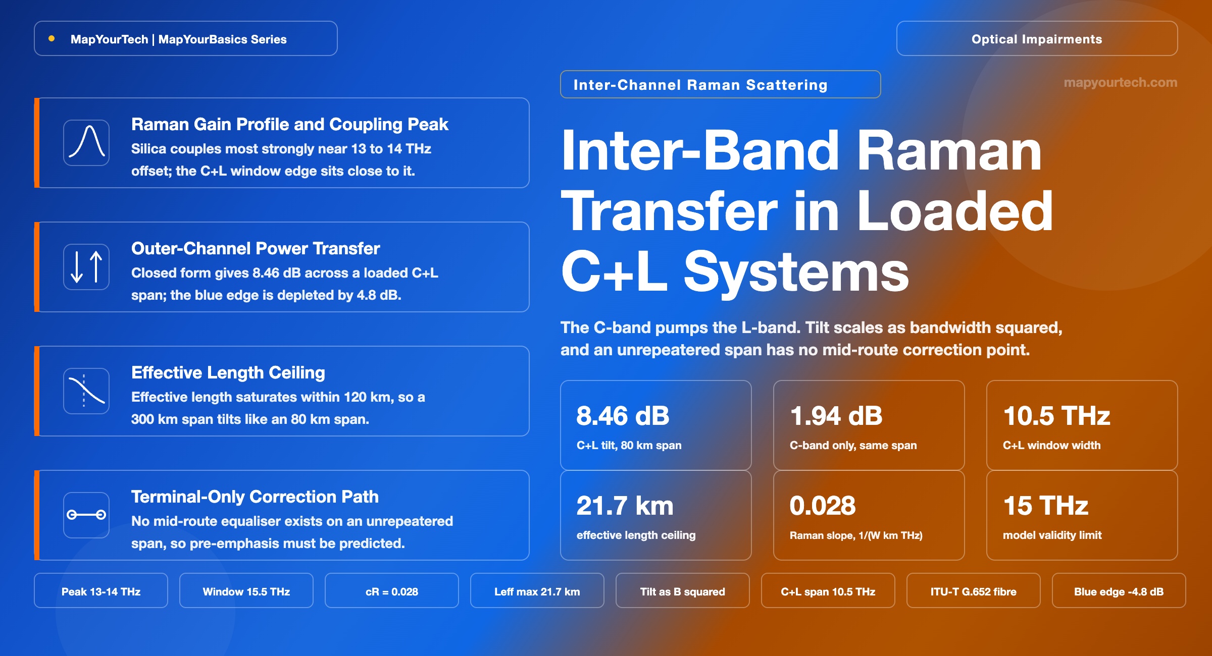
In a loaded C+L system the C-band channels are themselves Raman pumps for the L-band channels. The resulting tilt scales with the square of the occupied bandwidth, changes every time a channel is added, and on an unrepeatered span there is no mid-route element to correct it.
- Mechanism, quantification and mitigation
- Worked from the ISRS closed form
- Interactive tilt sandbox
Every bit matters, but how you transmit them matters more.
1. Introduction
Silica is not a passive medium for a wide optical comb. A photon at one frequency can scatter off a molecular vibration in the glass and emerge at a lower frequency, transferring energy as it goes, and in a wavelength-division-multiplexed system every channel is a candidate pump for every channel below it in frequency. The consequence is a permanent power gradient across the transmitted spectrum: short wavelengths are depleted, long wavelengths are amplified, and nothing in the fibre prevents it.
Inside the C-band alone this effect is a nuisance of roughly 1 to 2 dB that ordinary per-channel power setting absorbs. Extend the comb into the L-band and the same mechanism produces 8 to 14 dB of end-to-end power transfer, because two things change at once: the number of pump channels roughly doubles, and the frequency separation between the extreme channels grows from about 4.8 THz to more than 10 THz — which happens to land near the offset where the Raman gain of silica is strongest. The design of a C+L band DWDM system therefore begins from the position that the two bands are not independent resources but one Raman-coupled medium.
This article does three things. It quantifies the transfer from the closed-form expression used in the ISRS literature, so the scaling with power, bandwidth, span length and fibre type is visible rather than asserted. It shows why the tilt is a function of channel loading rather than a fixed property of the link, which is what makes it an operational problem and not only a design one. And it examines the case the mechanism is hardest in: an unrepeatered span, where the two terminals are the only places anything can be corrected.
2. Stimulated Raman Scattering as a Broadband Coupling Mechanism
Stimulated Raman scattering (SRS) transfers optical power from a higher-frequency wave to a lower-frequency wave through the vibrational modes of the glass. In an amplifier the effect is used deliberately: a pump launched roughly 100 nm below the signal wavelength produces gain in the transmission fibre itself, which is the basis of distributed Raman amplification. Between signal channels the same physics operates without being asked to, and the term for it is inter-channel stimulated Raman scattering (ISRS).
The governing relation for the power in channel i along the fibre contains three terms: ordinary attenuation, gain received from every channel above it in frequency, and depletion caused by every channel below it. Written out, the power evolution is a coupled set with one equation per channel, and the coupling coefficient between any pair is the Raman gain efficiency at their frequency separation.
Power moves from shorter wavelengths to longer wavelengths, equivalently from higher frequencies to lower. The higher-frequency channel acts as the pump and undergoes Raman depletion; the lower-frequency channel receives Raman gain. In a C+L system this means the C-band systematically transfers power to the L-band, the C-band blue edge is depleted most because it sits above the largest number of receivers at the largest separations, and the L-band red edge gains most. The effect is not a loss mechanism in aggregate — the power is redistributed rather than destroyed — which is why the L-band can end up with more power than it was launched with.
Two properties make ISRS awkward compared with the impairments it sits alongside. It is broadband: unlike four-wave mixing, which needs phase matching, Raman coupling exists between any pair of frequencies within roughly 15 THz regardless of dispersion. And it is load-dependent: the coupling strength is proportional to the power present in the pumping channels, so the impairment on an in-service channel is set by what else is lit.
3. The Raman Gain Profile and the Triangular Approximation
The Raman gain efficiency of silica as a function of frequency offset is not a simple shape. It rises from zero, reaches a principal maximum in the region of 13 to 14 THz, carries a shoulder just above that maximum, then falls away through a series of smaller features and is negligible beyond roughly 30 THz. For system modelling this profile is usually replaced by a straight line through the origin, cut off at a window edge:
gR(Δf) ≈ cR · Δf · H(ΔR − Δf)
Where: gR is the Raman gain efficiency in 1/(W·km); Δf is the frequency separation between the two channels in THz; cR is the slope of the linear fit in 1/(W·km·THz); H is the Heaviside discontinuous step; and ΔR is the window edge, taken in recent formulations as about 15.5 THz with the notional peak placed at 14 THz so that cR = GR/14 THz, with GR the peak Raman gain efficiency.
Practical Example — where the slope value comes from. A standard single-mode fibre with an effective area near 80 µm² has a peak Raman gain efficiency of roughly 0.40 1/(W·km). Dividing by a 14 THz peak offset gives cR ≈ 0.029 1/(W·km·THz), which is why values close to 0.028 are the ones commonly used in the ISRS modelling literature for this fibre class.
The approximation is worth understanding rather than accepting, because everything that follows inherits its behaviour. A linear gain profile means the coupling between two channels is proportional to how far apart they are, so the extreme pair in a comb is coupled most strongly and the tilt across the comb grows with the comb's width. It also means the model has a hard validity boundary: past the window edge the real profile turns over while the straight line keeps rising, so the approximation overstates the transfer for combs wider than about 15 THz. Section 15 returns to this.
4. Frequency Separation of the C+L Window Against the Gain Peak
The reason C+L behaves qualitatively differently from C-band alone is a coincidence of numbers. Taking a super-C band of about 4.8 THz and a super-L band of similar width with an inter-band gap at the splitter transition, the extreme channels of a C+L comb are separated by roughly 10.5 THz. The Raman gain of silica peaks near 13 to 14 THz. A C+L system therefore places its most widely separated channels close to the offset of maximum Raman coupling, while a C-band-only system at 4.8 THz sits low on the rising edge of the same profile, where the coupling efficiency is a fraction of its peak.
Reading the coupling efficiency at each window edge from the profile gives the first-order explanation for the magnitudes in the next section. At 4.8 THz the normalised efficiency is roughly a third of peak; at 10.5 THz it is close to three-quarters. Combined with roughly twice the aggregate pump power, that is where a factor of four to five in tilt comes from.
Takeaway: C+L is not simply twice as much spectrum as C-band. It is spectrum wide enough to reach the Raman coupling maximum, which is why the tilt grows faster than the bandwidth does.
5. Outer-Channel Power Transfer
The quantity that matters for design is the net transfer between the extreme channels of the comb: the Raman gain accumulated by the lowest-frequency channel added to the Raman depletion suffered by the highest-frequency channel. Inside the triangular region this has a closed form that is simple enough to reason with directly.
Δρ [dB] = 4.3 · Ptot · cR · Leff · Btot
Where: Δρ is the net power transfer between the outermost channels in dB; Ptot is the total launched power across the comb in W; cR is the Raman gain slope in 1/(W·km·THz); Btot is the total optical bandwidth in THz; and Leff = (1 − e−αL)/α is the effective length in km, with α the attenuation coefficient in 1/km and L the span length. The factor 4.3 converts the natural-log result to dB. The expression holds for bandwidths up to about 15 THz.
Practical Example — a C+L span at 80 km. With Ptot = 25 dBm (0.316 W), Btot = 10.5 THz, cR = 0.028 1/(W·km·THz) and α = 0.20 dB/km giving Leff = 21.17 km, the transfer is 4.3 × 0.316 × 0.028 × 21.17 × 10.5 = 8.46 dB. The split either side of the comb centre is not symmetric, because the redistribution profile is exponential in frequency rather than linear: the L-band red edge gains about 3.4 dB while the C-band blue edge is depleted by about 4.8 dB. The depleted edge always moves further than the amplified one.
The same fibre carrying C-band alone at 22 dBm across 4.8 THz gives 1.94 dB, so lighting the L-band on this span multiplies the outer-channel transfer by a factor of 4.4. That figure is consistent in sign and order with what a production planning tool reports for the same transition: a C-band to C+L capacity migration on an 80 km G.652.D span at comparable launch power costs the C-band roughly 2.7 dB of delivered generalised signal-to-noise ratio, with the shortest-wavelength channel losing more than 3 dB. The two numbers are not the same quantity — one is raw power transfer across the comb, the other is delivered GSNR after amplifier gain restoration — but the blue-edge depletion computed here is the mechanism that produces the reported GSNR loss.
The sandbox below evaluates the expression in both directions and exposes the fibre parameters separately, because Section 8 shows they do not move together. It opens on the worked example above.
6. Bandwidth-Squared Scaling at Constant Power Spectral Density
The closed form is linear in both Ptot and Btot, which looks benign until the two are connected. An operator widening a system does not hold total power constant; it holds power spectral density roughly constant, because per-channel launch power is set by the nonlinear optimum rather than by a total-power budget. Adding spectrum therefore adds power in proportion, and Ptot becomes proportional to Btot.
Δρ [dB] = 4.3 · ρ · cR · Leff · Btot2
Where: ρ = Ptot/Btot is the power spectral density in W/THz, held fixed as the comb widens. Substituting Ptot = ρBtot into the previous expression leaves the bandwidth appearing twice, once through the aggregate pump power and once through the frequency separation of the extreme pair.
Practical Example — widening a 300 km span at fixed density. At ρ corresponding to 22 dBm over 4.8 THz, the coefficient 4.3ρcRLeff evaluates to 0.086 dB/THz². The comb then produces 1.99 dB of transfer at 4.8 THz, 9.52 dB at 10.5 THz and 19.4 dB at 15 THz — a quadratic, not a proportional, penalty for spectrum.
Takeaway: Spectrum is not a linear purchase. At the constant power spectral density an operator runs in practice, doubling the occupied bandwidth roughly quadruples the outer-channel tilt, which is the arithmetic behind the observation that C+L is a different design problem rather than a wider one.
7. The Effective Length Ceiling and Span Length Independence
Effective length is the term that makes SRS behave unlike most accumulating impairments. Because the interaction strength is proportional to the product of the two channel powers, and both decay with distance, most of the transfer happens in the first few tens of kilometres. As the span lengthens, Leff = (1 − e−αL)/α saturates at its ceiling of 1/α.
| Span length | L (km) | Leff (km) | Percentage of 1/α ceiling |
|---|---|---|---|
| Short metro span | 40 | 18.27 | 84% |
| Typical amplified span | 80 | 21.17 | 97% |
| Long amplified span | 120 | 21.63 | 100% |
| Unrepeatered span | 300 | 21.71 | 100% |
| Long unrepeatered span | 500 | 21.71 | 100% |
The consequence is counterintuitive and worth stating plainly: a 300 km unrepeatered span generates almost exactly the same outer-channel tilt as an 80 km amplified span at the same launch power and bandwidth — 8.68 dB against 8.46 dB in the worked C+L case, a difference of 0.2 dB. Span length is not the variable that makes an unrepeatered system harder. The transfer is set by launch power, bandwidth and fibre properties, all of which are decided at the terminal.
It is tempting to assume an unrepeatered span suffers more Raman tilt because the light travels further without amplification. The effective-length ceiling says otherwise. The difficulty in an unrepeatered system is not the amount of tilt generated in one span; it is that there is no place between the two terminals to remove it, and that the amount generated changes with loading. Sections 9 through 12 develop that argument.
8. Fibre Choice: Attenuation Against Effective Area
Unrepeatered systems are built on low-attenuation, large-effective-area fibre, because both properties buy reach. Both also enter the tilt expression, and they pull in opposite directions, which makes this one of the places where a plausible-sounding conclusion is wrong.
- Lower attenuation raises the tilt. The effective-length ceiling is 1/α, so moving from 0.20 dB/km to 0.155 dB/km raises Leff from 21.71 km to 28.02 km, a 29% increase in interaction length and therefore in transfer.
- Larger effective area lowers the tilt. Raman gain efficiency scales inversely with effective area, so cR falls as the mode spreads. Moving from 80 µm² to 130 µm² reduces cR from 0.028 to roughly 0.017 1/(W·km·THz), a 38% reduction.
| Fibre class | α (dB/km) | Aeff (µm²) | cR | Leff (km) | Tilt (dB) |
|---|---|---|---|---|---|
| Standard single-mode | 0.200 | 80 | 0.0280 | 21.71 | 13.76 |
| Low-loss, large effective area | 0.155 | 130 | 0.0172 | 28.02 | 10.92 |
| Low loss with the slope held wrongly constant | 0.155 | 80 | 0.0280 | 28.02 | 17.75 |
The third row is the error worth avoiding. Treating cR as a fibre-independent constant and changing only the attenuation predicts a 29% increase in tilt, and would suggest that the fibre chosen for unrepeatered reach makes the Raman problem worse. Scaling the slope with effective area as the physics requires gives the opposite result: the low-loss large-area fibre produces about 21% less tilt than standard fibre, because the reduction in gain efficiency more than offsets the longer interaction length. Fibre selection for an unrepeatered span is therefore not a trade against Raman tilt — it happens to help on both counts.
Takeaway: The Raman gain slope is a property of the fibre, not a constant of the model. Any tilt comparison across fibre types that holds cR fixed while varying attenuation will get the sign of the answer wrong.
9. Load Dependence of the Tilt
Everything so far has assumed a fully loaded comb. In service that assumption fails almost immediately, and this is what turns ISRS from a design calculation into an operational constraint.
The transfer is proportional to Ptot, the power present in the fibre. A system provisioned to a 10.5 THz plan but running at 40% fill carries roughly 40% of the aggregate pump power, so it produces roughly 40% of the tilt. A pre-emphasis shape computed for full fill is then wrong by several decibels at the band edges. The reverse case is worse: a system commissioned at partial fill and pre-emphasised accordingly will drift as channels are added, and every channel added changes the operating point of every channel already in service. That is the effect behind the migration case cited in Section 5, where lighting the first L-band channel changes conditions for all 96 in-service C-band channels at once.
Which part of the spectrum is filled matters as much as how much of it. Because coupling is proportional to frequency separation, filling the L-band pumps nothing and is pumped by everything above it, while filling the C-band blue edge pumps the whole comb below it. Two systems at identical total power and identical channel count can therefore present quite different tilt if one is filled contiguously from the blue edge and the other from the red.
The established answer is to hold the spectral occupancy constant regardless of how many channels are carrying traffic, by filling unused slots with amplified spontaneous emission from the amplifier itself. The comb the fibre sees never changes, so the tilt never changes, and one pre-emphasis shape remains correct from commissioning to full fill. The cost is that the pump power spent on ASE is power not spent on traffic, and the loading must be maintained and monitored as a service-affecting function in its own right. On a system where the tilt is 1 to 2 dB this is optional; at 9 dB it is not.
10. Spectrum Evolution from C-Band to Equalised C+L
The mechanism, its magnitude and its load dependence are easier to hold together as a sequence than as three separate results. The stepped visual below walks one 80 km span through seven states: a C-band comb launched and received, the L-band lit alongside it, the uncorrected C+L spectrum, transmitter pre-emphasis and its result, and finally what receive-side equalisation alone achieves. Channel powers at every stage come from the same closed form used in Section 5, evaluated at 24 channels per band on a 200 GHz spacing. The three chips above the plots state what is on screen at any moment — which bands are lit, whether the spectrum is being viewed at the transmitter or after the span, and which correction is in force — so a stage can be read without tracking how it was reached.
Three things are worth watching for as the stages advance. The C-band-only tilt reads as almost flat at 1.86 dB across the comb, which is why the impairment was a second-order concern for three decades of C-band systems. Lighting the L-band takes the same span to 8.30 dB between its outermost channels without any parameter changing except occupancy. And the asymmetry is visible directly: the C-band blue edge falls 4.87 dB while the L-band red edge rises only 3.43 dB, because the redistribution profile is exponential in frequency.
Stages six and seven arrive at an identical flat received power spectrum by two different routes, and they are not equivalent. Pre-emphasis at the transmitter gives the channels that will be depleted their extra power before the span, so they accumulate noise against a higher signal level and their delivered OSNR is restored along with their power. Equalisation at the receiver attenuates whatever arrived strong, which levels the power display and leaves the OSNR gradient exactly where it was — the lower panel keeps its full tilt. A flat spectrum at the receive terminal is therefore not evidence that the impairment has been handled; it is only evidence that something was attenuated.
Section 5 gives 8.46 dB for this case and the visual reports 8.30 dB. The first is the band-edge-to-band-edge figure across the full 10.5 THz window that the closed form takes as Btot; the second is the transfer between the outermost populated channels, whose centres are 10.3 THz apart because the first and last slots sit inside the band edges. The visual also shows the pre-emphasis stage as an exact mirror of the received profile, which is a first-order construction: changing the launch shape changes the total power and therefore the transfer, so a real pre-emphasis shape is reached by iteration.
Takeaway: Nothing in the sequence changes except which slots are occupied. The span, the fibre, the per-channel launch density and the span loss are constant from stage one to stage four, and the tilt still grows by a factor of four and a half — which is the operational meaning of load dependence.
11. Tilt Correction on a Repeatered Line System
An amplified line system corrects tilt because it has somewhere to do it. Every amplifier site is an opportunity to reshape the spectrum, and the standard toolkit is well established: a gain-flattening filter fixes the amplifier's own gain shape, a dynamic gain equaliser or the per-channel attenuators inside a wavelength selective switch correct the accumulated spectral shape, and per-channel power control at the amplifier closes the loop against measured values.
The arithmetic of this arrangement is favourable in a way that is easy to miss. A ten-span link at 80 km per span generates roughly 8.5 dB of C+L tilt per span, so nearly 85 dB of raw transfer end to end — a figure that would be hopeless if it accumulated. It does not, because each site restores the shape before the next span begins. What accumulates is the residual error of each correction, which is small, plus the noise penalty of having amplified a depleted channel back to nominal. The number that reaches the receiver is a few decibels of GSNR gradient, not tens of decibels of power gradient.
Two further advantages follow from having mid-route elements. Correction is adaptive: a per-channel control loop reacting to measured power tracks a change in loading automatically, so partial fill and channel additions are handled without recomputing anything at the transmitter. And correction is distributed, so no single element has to impose a large shape, which keeps the required dynamic range of each equaliser modest. A C+L line system depends on both properties, and the same reasoning drives gain-shaping choices inside submarine repeater design, where distributed Raman has been used to widen repeater spacing and dynamic tilt control removes the need for submerged gain equalisers.
12. Terminal-Only Correction on an Unrepeatered Span
An unrepeatered span removes every one of those elements. There is no amplifier site, therefore no gain-flattening filter, no dynamic gain equaliser and no wavelength selective switch anywhere between the two cable landing stations. The correction points are the transmit terminal and the receive terminal, and nothing else.
Three consequences follow, and they compound.
- The correction is open-loop at the transmitter. Pre-emphasis has to be computed for a predicted loading and launched blind. On an amplified system a control loop measures the result and adjusts; here the transmitter cannot see the receive spectrum except through management-plane feedback across the span, which is slow and coarse by comparison.
- The receive terminal can equalise power but not recover signal-to-noise ratio. Flattening a spectrum at the receiver by attenuating the channels that arrived strong does nothing for the channels that arrived weak. The depleted C-band blue edge has already accumulated its noise penalty, and the equaliser only makes the result uniform, not better.
- The remote amplifier cannot help. A remote optically pumped amplifier contributes gain with its own wavelength dependence, fixed at design time, with no telemetry and no in-service adjustment. It is one more fixed shape in the cascade rather than a correction opportunity.
Takeaway: The tilt an unrepeatered span generates is ordinary. What is not ordinary is that it must be predicted before launch, cannot be measured mid-route, and cannot be adjusted after the cable is on the sea bed — which is why ASE loading and worst-case design carry so much weight in this class of system.
13. Coupling Between Signal Tilt and Distributed Raman Pump Gain
An unrepeatered span at 60 dB or more of loss uses distributed Raman pumps at watt-level power, and those pumps interact with the same mechanism. Three couplings arise, and none is separable from the others.
- Pump-to-signal gain is wavelength dependent by design. A pump set chosen to produce a flat gain profile across C-band produces a different profile across C+L, because the offset from each pump to each channel differs. Shaping Raman gain to oppose the signal tilt is possible and is done — a pump can be positioned to give more gain to the depleted blue edge — but the same pumps then also interact with the L-band channels through their own Raman process, so the correction is not independent of the impairment it removes.
- Signal-to-pump depletion. At high signal power the comb depletes the pumps, so the achieved on-off Raman gain depends on how the comb is loaded. Gain that was characterised at full fill will be different at partial fill, in the opposite direction to the signal tilt change.
- Pump-to-pump transfer. Where several pump wavelengths are used to broaden or shape the gain, the shorter-wavelength pumps pump the longer-wavelength ones, so the pump powers arriving in the fibre are not the powers launched.
The practical effect is that the gain profile and the tilt are one coupled problem with a single solution rather than two effects to be corrected in sequence. This is the reason C+L support on the high-power Raman used for the longest unrepeatered spans is not simply a matter of adding pump wavelengths, and why C-band-only operation remains common in that equipment class even where the line system itself supports both bands.
14. Design Consequences and Mitigation Practice
The Binding Channel
Because depletion is worst where the frequency separation to the rest of the comb is largest, the binding channel in a C+L design is the C-band blue edge. It carries the largest Raman depletion, and it sits at the shortest wavelength, where fibre attenuation is also highest. A design that meets its target at the blue edge meets it everywhere, which is why worst-case channel selection rather than average performance drives the modulation and rate plan. The published treatment of band allocation in C+L design puts the resulting GSNR gradient at 3.5 dB or more and treats it as a permanent design input rather than a fault to be removed.
The L-Band Is Not Uniformly Worse
It is easy to assume the L-band is the disadvantaged band because its amplifiers have higher noise figure and its fibre attenuation is higher at the red edge. Raman transfer works the other way: the L-band receives power the C-band gives up, which partly offsets its amplifier penalty. Whether the L-band ends up better or worse than the C-band on a given link is the outcome of that competition, not a property that can be assumed, and it is one of the reasons per-channel OSNR and rate assignment has to come from a model rather than from a rule of thumb.
Mitigation, in the Order It Is Usually Applied
- ASE loading to hold spectral occupancy constant, so the tilt is a fixed quantity the design can be built around rather than a moving one.
- Transmitter pre-emphasis shaped for the loaded condition, so the spectrum arriving at the receiver is closer to flat than the spectrum launched.
- Raman pump shaping to place gain preferentially where depletion is worst, accepting the coupling described in Section 13.
- Launch power reduction as the direct lever, since the tilt is proportional to Ptot. The inverse tab of the sandbox gives the trade explicitly: holding the outer-channel transfer to 3 dB across 10.5 THz on a 300 km standard-fibre span caps total launch at about 20.4 dBm, which is well below the nonlinear optimum — so tilt and nonlinearity are competing constraints on the same variable.
- Band allocation and rate assignment as the last resort, accepting the gradient and assigning lower rates to the channels that sit at the wrong end of it.
For planning purposes the effect has to be inside the model rather than applied as a margin afterwards. Tools that carry an ISRS correction in the Gaussian noise model report per-channel GSNR agreement within about 0.5 dB of measurement on C+L systems, and the ISRS closed form used here sits within roughly 0.2 dB of split-step simulation on nonlinear interference power — which is the standard of accuracy an in-house multivendor planning capability needs before it can be trusted to set rates.
15. Validity Limits of the Triangular Model
Every figure in this article comes from the triangular approximation, and it has a boundary. The closed form is valid for total optical bandwidths up to about 15 THz, because that is where the linear fit to the Raman gain profile stops being a fair description. Two things happen beyond it.
The real profile turns over. The Raman-induced tilt reaches a maximum at a total optical bandwidth of roughly 15 THz, slightly wider than the Raman frequency shift itself, and decreases beyond that — while the triangular expression keeps rising without limit. Any figure this model produces past 15 THz overstates the transfer, which is why the shaded region of Figure 2 is marked rather than extrapolated.
The shape also stops being monotonic. In S+C+L or C+L+U systems the coupling between a given pair depends on where both sit relative to the gain peak and its shoulders, so the tilt across the comb is no longer a simple gradient from blue to red. Measurements on C+L+U systems show that the triangular approximation introduces errors at both edges of the spectrum and that an accurate Raman gain coefficient spectrum is required instead.
The same boundary shapes what a change of transmission medium would buy. A fibre whose low-loss window is both wider and far less Raman-active changes the problem rather than the parameters, which is part of the interest in hollow core fibre for wideband transmission: guiding in air removes most of the glass the Raman interaction depends on.
C+L at roughly 10.5 THz sits inside the valid region, so the 8 to 14 dB figures are usable. They are, however, close to the boundary: a system extending into super-L or adding a guard-band-free S-band allocation moves past it, and the model has to be replaced rather than extended. Anyone carrying these results into a multiband design should treat 15 THz as a hard line and switch to the measured gain spectrum on the far side of it.
16. Conclusion
Inter-band Raman transfer is the clearest case in optical transmission of an impairment that is not a defect. It is a property of glass, it operates on every wide comb, and it cannot be engineered out — only accounted for. What makes it worth understanding quantitatively is that its scaling is unfriendly in a specific way: at the constant power spectral density operators run in practice, the outer-channel transfer grows with the square of the occupied bandwidth, so the step from C-band to C+L multiplies it by roughly four and lands the extreme channel pair close to the offset where silica couples most strongly.
The span-length result is the one most likely to be assumed wrongly. Effective length saturates at 1/α within about 120 km, so a 300 km unrepeatered span generates the same per-span tilt as an 80 km amplified span to within 0.2 dB. The difficulty in an unrepeatered system is structural rather than physical: the correction elements that make a repeatered line system tractable — gain-flattening filters, dynamic gain equalisers, per-channel control loops that adapt to loading — are all mid-route elements, and an unrepeatered span has no mid-route. Pre-emphasis has to be computed for a loading that has not occurred, the remote amplifier contributes fixed gain with no adjustment, and the receive terminal can flatten a spectrum without recovering the signal-to-noise ratio already lost.
Two results here contradict a plausible first guess and are worth carrying away. Low-loss large-effective-area fibre reduces the tilt rather than increasing it, because the fall in Raman gain efficiency with mode area more than offsets the longer effective length — provided the gain slope is scaled with the fibre rather than held constant. And the L-band is not uniformly the disadvantaged band, because it receives the power the C-band gives up. The binding channel is the C-band blue edge, in every case, and a C+L design that holds there holds everywhere.
17. References
- D. Semrau, R. I. Killey and P. Bayvel, A Closed-Form Approximation of the Gaussian Noise Model in the Presence of Inter-Channel Stimulated Raman Scattering, Journal of Lightwave Technology.
- D. Semrau, R. I. Killey and P. Bayvel, Inter-channel Stimulated Raman Scattering and its Impact in Wideband Transmission Systems, Optical Fiber Communication Conference.
- H. Rabbani, G. Liga, V. Oliari, L. Beygi, E. Agrell, M. Karlsson and A. Alvarado, A General Analytical Model of Nonlinear Fiber Propagation in the Presence of Kerr Nonlinearity and Stimulated Raman Scattering, Journal of Lightwave Technology.
- Raman-Induced Power Tilt in Arbitrarily Large Wavelength-Division-Multiplexed Systems, IEEE Photonics Technology Letters.
- Accurate Estimation of Inter-channel Stimulated Raman Scattering in C+L+U Ultra-wideband WDM Systems beyond Raman Shift Frequency, IEEE.
- Closed-form Expression for the Power Profile in Wideband Systems with Inter-channel Stimulated Raman Scattering, arXiv.
- A. R. Chraplyvy, Limitations on Lightwave Communications Imposed by Optical-Fiber Nonlinearities, IEEE Journal of Lightwave Technology.
- ITU-T Recommendation G.694.1, Spectral grids for WDM applications: DWDM frequency grid, ITU-T Study Group 15.
- ITU-T Recommendation G.652, Characteristics of a single-mode optical fibre and cable, ITU-T Study Group 15.
Sanjay Yadav, "Optical Network Communications: An Engineer's Perspective" — Bridge the Gap Between Theory and Practice in Optical Networking.
Related Articles on MapYourTech