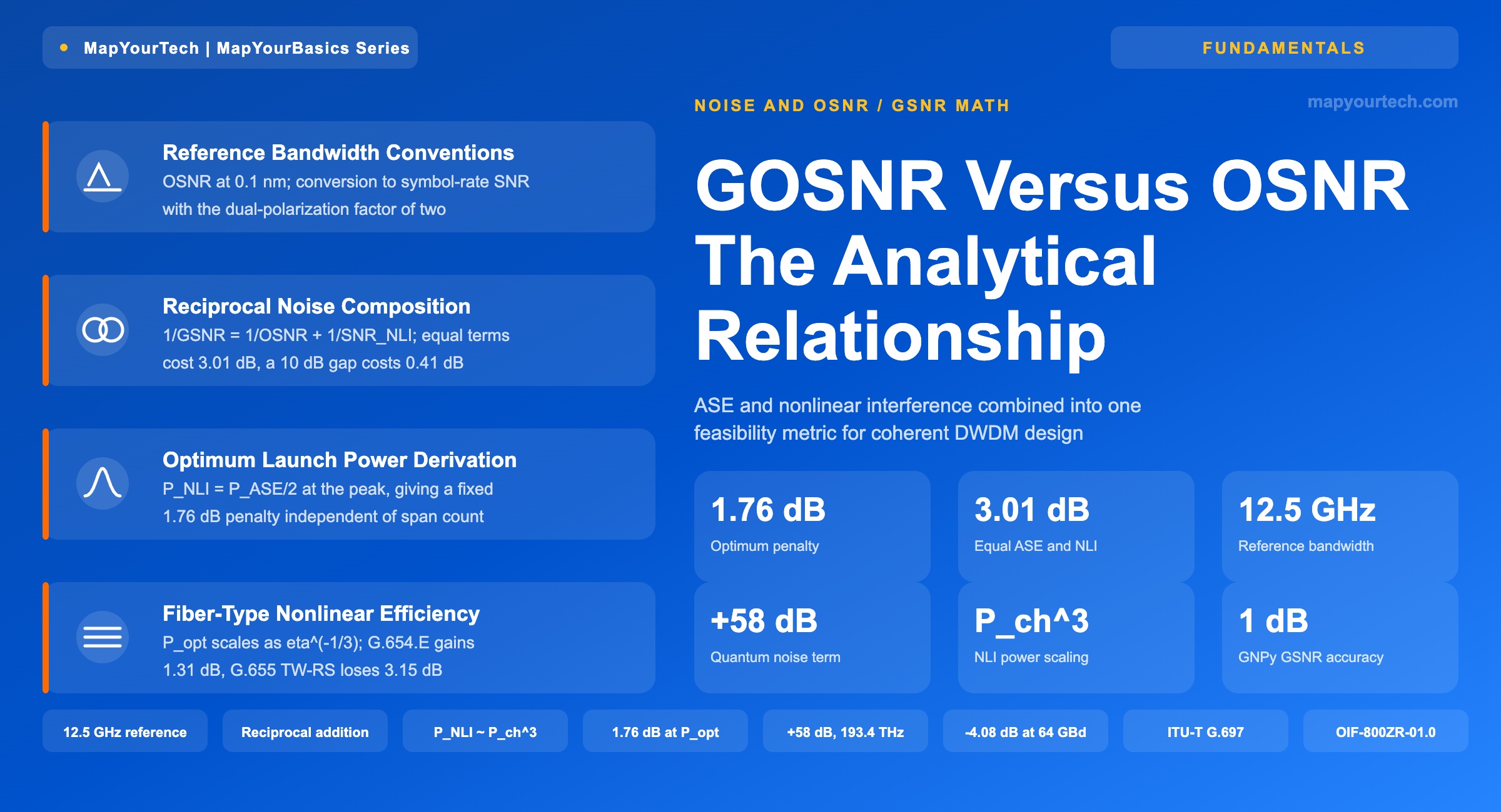
GOSNR Versus OSNR: The Analytical Relationship
How amplified spontaneous emission and nonlinear interference combine into a single feasibility metric, and what the composition rule implies for launch power, fiber type, and receiver margin.
1. Introduction
A planning tool that reports 22 dB optical signal-to-noise ratio (OSNR) on a 1,200 km path and a receiver that reports 19 dB signal-to-noise ratio (SNR) are not in disagreement. They are measuring two different quantities. OSNR counts amplified spontaneous emission (ASE) from the amplifier chain and nothing else. The coherent receiver's digital signal processing (DSP) block sees ASE plus the Kerr-generated nonlinear interference (NLI) accumulated in every fiber span, and it cannot distinguish the two because, in an uncompensated link, both behave as additive white Gaussian noise.
Generalized OSNR — written GOSNR in vendor planning tools and GSNR in the Gaussian Noise (GN) model literature — is the metric that reconciles them. It is the quantity dense wavelength division multiplexing (DWDM) planning tools compare against a transceiver threshold to declare a lightpath feasible, and the quantity a digital twin reconciles against live telemetry. This article derives the composition rule that links the two, the cubic power scaling that makes NLI behave unlike ASE, the resulting 1.76 dB penalty at optimum launch power, and the reference-bandwidth conversion that turns either figure into the receiver SNR a transceiver datasheet is written against. Readers who want the underlying noise accounting first should start with the OSNR fundamentals primer.
2. Definitions and Reference Bandwidth Conventions
OSNR is the ratio of per-channel signal power to ASE noise power measured in a reference bandwidth. ITU-T G.697 fixes that reference at 0.1 nm, which corresponds to 12.5 GHz near 1550 nm — a standard-specified convention, and the reason optical spectrum analyser readings are comparable across vendors. GSNR uses the same signal power in the numerator and adds the nonlinear interference power to the denominator, referred to the same bandwidth.
OSNR  =  P_ch / P_ASE                        (linear ratio, 12.5 GHz reference)
GSNR  =  P_ch / ( P_ASE + P_NLI )                (same reference bandwidth)

P_ch  = per-channel optical power, mW
P_ASE = accumulated amplified spontaneous emission power, mW
P_NLI = accumulated nonlinear interference power, mW

GSNR (dB) = 10*log10( P_ch / (P_ASE + P_NLI) )
The receiver, however, does not work in a 12.5 GHz window. It works over the signal bandwidth, and for a dual-polarization signal the ASE in both polarizations reaches the detector. Converting a 0.1 nm figure to the electrical SNR the DSP reports requires a bandwidth term:
SNR (dB)  =  GSNR (dB)  +  10*log10( 2 * B_ref / R_s )

B_ref = 12.5 GHz reference bandwidth (0.1 nm at 1550 nm)
R_s   = channel symbol rate, GBd
factor 2 accounts for both polarizations of a DP signal| Symbol Rate | Representative Interface | Conversion Term (dB) |
|---|---|---|
| 32 GBd | 100G DP-QPSK | -1.07 |
| 45 GBd | 200G DP-16QAM | -2.55 |
| 64 GBd | 400G DP-16QAM, 400ZR class | -4.08 |
| 96 GBd | 800G DP-16QAM, short reach | -5.84 |
| 118.2 GBd | 800ZR per OIF-800ZR-01.0 | -6.75 |
The 118.203 GBd figure is standard-specified: OIF-800ZR-01.0, released 30 October 2024, defines an 800G coherent line interface using DP-16QAM at that nominal baud rate with oFEC for single-span amplified 80–120 km links. The conversion terms in Table 1 are arithmetic consequences of the formula above.
Takeaway: A GSNR figure without its reference bandwidth is unusable. Compare 0.1 nm values against 0.1 nm transceiver thresholds, or convert both to symbol-rate SNR — never mix the two conventions in one budget.
3. Reciprocal Composition of ASE and Nonlinear Noise
Because both noise terms are treated as additive and statistically independent, their powers add directly, which means their inverse signal-to-noise ratios add. Dividing the GSNR definition through by the channel power gives the composition rule used in every GN-model implementation:
1 / GSNR  =  1 / OSNR_ASE  +  1 / SNR_NLI        (all terms linear)

OSNR_ASE = P_ch / P_ASE   ... the ASE-only ratio
SNR_NLI  = P_ch / P_NLI   ... the NLI-only ratio

GSNR_dB = -10*log10( 10^(-OSNR_dB/10) + 10^(-SNR_NLI_dB/10) )
The structure is the same as parallel resistance: the smaller term dominates. When the two contributions are equal, GSNR sits 3.01 dB below either one. When they differ by 10 dB, the larger contributor costs only 0.41 dB. This asymmetry is why chasing a 1 dB amplifier noise figure improvement on a link that is already nonlinearity-limited returns almost nothing, and why the two terms must be tracked separately rather than lumped into a single margin allowance. The Gaussian Noise model treatment develops the spectral-domain derivation behind the NLI term.
4. Nonlinear Interference Scaling and Optimum Launch Power
ASE power is set by amplifier gain, noise figure and span count. It does not depend on the channel power at all, so OSNR_ASE rises 1 dB for every 1 dB of added launch power. Nonlinear interference behaves differently: under the GN model the NLI power grows as the cube of the channel power, so SNR_NLI falls 2 dB for every 1 dB added. The two mechanisms pull in opposite directions and there is a single power that maximises GSNR.
P_NLI  =  eta * P_ch^3            eta = NLI efficiency, mW^-2, per path

GSNR(P_ch) = P_ch / ( P_ASE + eta*P_ch^3 )

set d(GSNR)/d(P_ch) = 0:
        P_ASE + eta*P_ch^3 - 3*eta*P_ch^3 = 0
   -->  P_NLI  =  P_ASE / 2        at the optimum
   -->  P_opt  =  ( P_ASE / (2*eta) )^(1/3)

total noise at optimum = 1.5 * P_ASE, so:
   GSNR_max  =  (2/3) * OSNR_ASE   -->   1.76 dB below the ASE-only value
Two results follow that are worth holding on to. First, the nonlinear penalty at the optimum operating point is a fixed 1.76 dB — a theoretical limit of the GN model, independent of fiber type, span count and amplifier noise figure. Second, because both P_ASE and eta scale linearly with the number of identical spans, their ratio does not, so the optimum per-channel launch power is independent of path length to first order. This is the analytical basis for the local-optimisation approach used in planning tools: set each span to its own optimum and the end-to-end result is close to optimal. Shannon capacity bounds for fiber take the same 1.76 dB result as the starting point for the nonlinear capacity ceiling.
| Launch Power (dBm) | OSNR_ASE (dB) | GSNR (dB) | Penalty (dB) |
|---|---|---|---|
| -4 | 23.00 | 22.86 | 0.14 |
| -3 | 24.00 | 23.73 | 0.27 |
| -2 | 25.00 | 24.49 | 0.51 |
| -1 | 26.00 | 25.03 | 0.97 |
| 0 | 27.00 | 25.24 | 1.76 |
| 1 | 28.00 | 24.99 | 3.01 |
| 2 | 29.00 | 24.24 | 4.76 |
| 3 | 30.00 | 23.03 | 6.97 |
| 4 | 31.00 | 21.49 | 9.51 |
Takeaway: The GSNR curve is asymmetric. One decibel below optimum costs 0.21 dB of GSNR; one decibel above costs 0.25 dB and the gap widens fast. When span loss is uncertain, target slightly under the calculated optimum.
5. Propagation Rules for ASE and Nonlinear Noise
Tracking GSNR along a path requires carrying both noise terms as separate state variables and applying different rules to each at every element. The distinction is physical: an amplifier both generates and amplifies ASE, but it only amplifies the nonlinear interference already present; a transmission fiber attenuates both and generates new NLI in proportion to the cube of the power launched into it.
Because gain and loss act identically on signal and noise, no passive element between the amplifiers changes GSNR. Only two things move the number: the noise figure and gain of each amplifier, and the power launched into each fiber span. Every other component in the path is neutral to first order.
6. Practical Example — five-span GSNR budget at 64 GBd
Take a 400 km path of five identical 80 km G.652.D spans at 0.20 dB/km, giving 16 dB span loss, each followed by an erbium-doped fiber amplifier (EDFA) with a 5 dB noise figure. The channel is 64 GBd DP-16QAM. The ASE-only figure follows from the standard cascade relation, where the +58 dB constant is the magnitude of the quantum noise floor h·ν·B_ref at 193.4 THz over 12.5 GHz.
OSNR_ASE = P_ch - NF - L_span + 58 - 10*log10(N)

P_ch = 0 dBm, NF = 5 dB, L_span = 16 dB, N = 5 spans
   OSNR_ASE = 0 - 5 - 16 + 58 - 6.99 = 30.01 dB
The NLI-only ratio for the same path, evaluated with an efficiency coefficient calibrated so that the optimum launch power lands at 0 dBm, is 33.02 dB. Applying the composition rule gives a GSNR of 28.25 dB — the expected 1.76 dB below the ASE-only figure, because 0 dBm is the optimum here. The interesting comparison is what happens when a designer raises launch power by 2 dB to buy OSNR margin.
| Parameter | 0 dBm | +2 dBm | Change (dB) |
|---|---|---|---|
| ASE-only OSNR | 30.01 | 32.01 | +2.00 |
| NLI-only SNR | 33.02 | 29.02 | -4.00 |
| GSNR at 0.1 nm | 28.25 | 27.25 | -1.00 |
| Nonlinear penalty | 1.76 | 4.76 | +3.00 |
| Receiver SNR at 64 GBd | 24.17 | 23.17 | -1.00 |
Two decibels of extra launch power buys exactly 2 dB of OSNR and costs 1 dB of GSNR. A design review that signs off on the OSNR column alone approves a change that degrades the link. Against a required OSNR near 21–23 dB for 400G DP-16QAM at the 0.1 nm reference — a widely published transceiver-class figure rather than a single vendor specification — the 0 dBm case retains roughly 5–7 dB of end-of-life margin. The EDFA noise figure treatment covers the ASE half of this budget in more detail, and cascaded-span OSNR calculation generalises the +58 dB relation to unequal spans.
Takeaway: Report OSNR and GSNR side by side in every design review. A launch power change that improves one and degrades the other is invisible in a single-column budget.
7. Fiber-Type Dependence of Nonlinear Efficiency
The efficiency coefficient eta depends on the fiber's nonlinear coefficient, effective area, dispersion and attenuation. Low chromatic dispersion increases the phase-matching window for four-wave mixing and cross-phase modulation, so non-zero dispersion-shifted fibers generate substantially more NLI than standard single-mode fiber at the same launch power. Large effective area fibers generate less. Commercial planning tools encode this as a per-fiber-type coefficient; the ratios below are drawn from that class of coefficient set and are a planning-tool value rather than a measured constant.
Both the optimum launch power and the GSNR achieved at it shift by the same amount, because P_opt scales as eta^(-1/3) and GSNR_max is proportional to P_opt:
| Fiber Type | Relative NLI Efficiency | Shift in P_opt (dB) | Shift in GSNR_max (dB) |
|---|---|---|---|
| G.652.D standard single-mode | 1.00 | 0.00 | 0.00 |
| G.654.E large effective area | 0.40 | +1.31 | +1.31 |
| G.655 LEAF class | 4.52 | -2.19 | -2.19 |
| G.655 TW-Reach class | 7.62 | -2.94 | -2.94 |
| G.655 TW-RS class | 8.81 | -3.15 | -3.15 |
A path that mixes G.652.D and G.655 sections needs its optimum power set per span, not once for the route. The G.654.E column explains why large effective area fiber is selected for long submarine and terrestrial ultra-long-haul routes: the roughly 1.3 dB GSNR advantage compounds with its lower attenuation. The spectral efficiency levers discussion places this alongside baud rate and modulation choices.
8. Validity Boundaries and Design Guidelines
The GN model treats the WDM signal as statistically Gaussian. That holds once chromatic dispersion has decorrelated the channel phases, typically within the first two to three spans of an uncompensated coherent link. For G.652.D at 17 ps/(nm·km), one 80 km span accumulates 1,360 ps/nm, enough to satisfy the assumption for baud rates above roughly 25 GBd. The model degrades for low-dispersion fiber and for narrow-band, low-baud-rate carriers, where the enhanced GN model with modulation-format-dependent corrections is the appropriate refinement.
Three boundaries matter operationally:
- Dispersion-compensated links. Where dispersion compensating fiber (DCF) is present, the additive Gaussian assumption does not apply and GSNR is not defined. Planning tools return the parameter as not-applicable for any path traversing a DCF module.
- First-span accuracy. In the first one or two spans the GN model overestimates self-channel interference, so early-span GSNR predictions are pessimistic by a fraction of a decibel.
- Wideband operation. Across C+L band, inter-channel stimulated Raman scattering transfers power between bands and must be included; the ISRS-GN closed form reports an average deviation near 0.2 dB in NLI power against split-step simulation for standard single-mode fiber spans across the full C+L band — a published simulation-validated figure.
For threshold setting, commercial planning tools apply a GSNR threshold offset below the transceiver's OSNR threshold, typically in the range of 0.7–1.0 dB depending on release — a vendor planning-tool convention that absorbs the modelling uncertainty rather than a standard-specified value. Against measured plant, GNPy has been validated by operators to within roughly 1 dB of measured GSNR for more than 90% of experimental cases. Closing the residual gap is the job of a calibration loop; see digital twin calibration against measured GSNR and the wider in-house multivendor planning tool architecture. Monitoring practice for the measured side is covered in DWDM channel monitoring with OCM and OSA, and the modelling-versus-live-plant distinction in digital twin versus simulator.
Takeaway: GSNR is a model output, not a measurement. Quote it with its model assumptions and its calibration status, and hold design margin against the residual model error rather than assuming the number is exact.
9. Summary
OSNR counts ASE only; GSNR adds nonlinear interference in the same reference bandwidth. The two combine reciprocally, so the smaller of the ASE-only and NLI-only ratios dominates and equal contributions cost 3.01 dB. Nonlinear interference grows as the cube of channel power while ASE is independent of it, producing a single optimum launch power at which NLI power equals half the ASE power and GSNR sits a fixed 1.76 dB below the ASE-only figure. Because both terms scale with span count, that optimum is largely independent of path length.
Quick reference values: 12.5 GHz (0.1 nm) reference bandwidth; +58 dB quantum noise constant at 193.4 THz; -4.08 dB conversion from 0.1 nm GSNR to 64 GBd receiver SNR; 1.76 dB nonlinear penalty at optimum; 3.01 dB when ASE and NLI contribute equally; 21–23 dB required OSNR for 400G DP-16QAM. For deeper treatment, the Gaussian Noise model primer covers the spectral derivation and the OSNR fundamentals primer covers the ASE cascade.
References
- ITU-T G.697 — Optical monitoring for dense wavelength division multiplexing systems, ITU-T Study Group 15.
- P. Poggiolini, The GN Model of Non-Linear Propagation in Uncompensated Coherent Optical Systems, IEEE/OSA Journal of Lightwave Technology.
- Telecom Infra Project OOPT/PSE, GNPy — Route Planning and Optical Simulation Library, Telecom Infra Project.
- OIF-800ZR-01.0 — 800ZR Implementation Agreement, Optical Internetworking Forum.
- Sanjay Yadav, "Optical Network Communications: An Engineer's Perspective" — Bridge the Gap Between Theory and Practice in Optical Networking.
Related Articles on MapYourTech