Digital Twin Calibration Loops: Reconciling Predicted and Measured GSNR
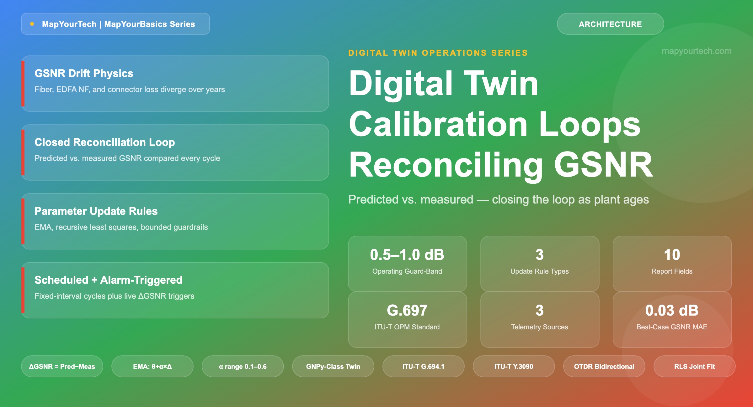
Turning twin calibration into a scheduled operational loop — the reconciliation report format and the parameter update rules that keep the model honest as the plant ages.
1. Introduction
A GNPy-class digital twin predicts the generalized signal-to-noise ratio (GSNR) of every lightpath in a network from a model of fiber loss, amplifier gain, and nonlinear interference. On day one, right after commissioning, that prediction typically tracks the coherent transceiver's measured GSNR within a decibel or better, because the model was built from the same span-loss and amplifier data used to turn the system up. Three years later, after two fiber repairs, one amplifier card swap, a connector re-termination, and a slow rise in splice loss from routine maintenance, the same model can be off by 2 to 3 dB on some spans — enough to erase the design margin on a channel running close to its forward error correction (FEC) threshold.
The twin did not get worse at math. The plant it describes moved, and nothing told the twin. Digital twin calibration loops close that gap: a scheduled, repeatable process that pulls measured GSNR and per-span telemetry from the live network, compares it against what the model predicted, and updates the model's parameters — fiber attenuation coefficients, amplifier noise figure curves, connector loss estimates — so the next prediction is closer to reality than the last one.
This article treats calibration as an operational process, not a one-time commissioning step. It covers the physical basis for why predicted and measured GSNR diverge, the architecture of a recurring calibration loop, the fields a reconciliation report needs to be useful to an operations team, and the update rules — exponential smoothing, recursive least squares, and threshold-gated re-fitting — that turn a residual error into a corrected parameter without letting a single bad measurement destabilize the model. The GN-model literature and field-verification studies referenced throughout are the same body of work behind the open-source GNPy planning tool and the commercial digital twins built on the same physics.
Scope: This article assumes familiarity with the Gaussian Noise (GN) model and GSNR as a quality-of-transmission (QoT) metric. Readers new to the underlying physics should first read the Gaussian Noise model primer and OSNR fundamentals before continuing.
2. Fundamentals: GSNR and the Two Numbers That Should Agree
GSNR folds every impairment that degrades a coherent channel's demodulation quality into a single figure: amplified spontaneous emission (ASE) from every optical amplifier in the path, and nonlinear interference (NLI) generated by the Kerr effect as channels co-propagate through fiber. Both are combined as noise-equivalent power referred to the signal, so a single number expresses the margin a transceiver has above its FEC threshold. In the GN-model formulation used throughout the optical networking literature, GSNR is expressed as signal power divided by the sum of these two noise contributions:
GSNR = P / ( σ²ASE + σ²NLI )

Equivalently, in reciprocal form:

1 / GSNR = 1 / OSNRASE + 1 / SNRNLI
Two independent instances of this quantity exist for every lightpath at every moment. The predicted GSNR is what the digital twin computes from its stored model of the plant: fiber attenuation coefficient per span, effective area and nonlinear coefficient of the deployed fiber type, each amplifier's gain and noise figure at its current operating point, and the channel loading assumed for the calculation. The measured GSNR is what the coherent transceiver's digital signal processor (DSP) reports from the live signal — derived from pre-FEC bit error rate (BER) via the transceiver's calibrated BER-to-GSNR curve, or from a dedicated GSNR estimation algorithm running on receiver-side telemetry. A 2026 OFC paper from NEC Labs America demonstrated deriving GSNR directly from BER telemetry combined with progressive receiver-side ASE loading, explicitly framing the technique as an enabler for digital-twin calibration in production metro networks.
On a healthy, freshly calibrated link these two numbers agree within the model's design tolerance — commonly under 1 dB for a well-characterized OLS. The gap between them, ΔGSNR = GSNRpredicted − GSNRmeasured, is the single quantity the entire calibration loop exists to drive back toward zero. A positive ΔGSNR means the model is optimistic — it thinks the link is better than it is, which is the dangerous direction, because it erodes real margin without warning. A negative ΔGSNR means the model is pessimistic, which wastes capacity but does not create outages.
Why the two numbers drift apart
Three mechanisms account for nearly all field-observed GSNR drift, and each has a distinct signature in a reconciliation report:
- Fiber attenuation drift. Splice loss increases slowly from thermal cycling and mechanical stress on closures; a single re-splice after a cut can add 0.05–0.3 dB at a point the model has no record of. This shows up as a per-span loss coefficient that no longer matches the fiber-type default the model was built with.
- Amplifier parameter drift. EDFA noise figure and gain-versus-tilt behavior shift with pump laser aging and gain-medium degradation over years of operation. A field study of semi-automatic line-system provisioning demonstrated that per-amplifier noise-figure-versus-gain curves extracted from live optical line system (OLS) measurements diverge measurably from the vendor default curves the model shipped with, and that feeding the extracted curves back into GNPy materially improved GSNR prediction accuracy.
- Topology and connector changes. Patch-panel re-terminations, ROADM add/drop reconfiguration, and connector cleaning (or the lack of it) change insertion loss at points the model may still hold at commissioning-time defaults.
Takeaway: GSNR drift is not a single failure mode — it is the sum of many small, physically distinct changes across fiber, amplifiers, and connectors. A calibration loop that treats ΔGSNR as one undifferentiated error cannot correct it; the loop has to decompose the residual by span and by component before it can update the right parameter.
3. Technical Architecture: The Calibration Loop
A calibration loop is structurally two parallel pipelines that meet at a comparison point. One pipeline produces the predicted GSNR from the stored model; the other produces the measured GSNR from live telemetry. Both run on the same schedule, feed a reconciliation engine that computes the per-span and per-channel residual, and — when that residual exceeds an operating guard-band — hand the result to a parameter update engine that writes corrected values back into the model store, closing the loop for the next cycle.
Three architectural decisions in this loop matter more than the specific software that implements them:
- The predicted and measured pipelines are decoupled from each other except at the reconciliation engine. The predictor does not need the live network to be reachable to run a hypothetical recompute, and the telemetry collector does not need the model to be current to gather a reading. This separation is what makes the loop resilient to partial outages in either subsystem.
- The decision gate is explicit, not implicit. A residual inside the guard-band produces no model change — this is a design choice, not an oversight. Auto-applying every measurement as a parameter update would let a single noisy reading (a transceiver briefly training after a protection switch, an OTDR trace taken during a splice repair) corrupt the model. The gate is what separates a calibration loop from naive online learning.
- The reconciliation report is a first-class output, not a debug log. It is what an operations team reads to understand why the model changed, and it is the audit trail that lets an engineer roll back a bad update.
3.1 The Reconciliation Report Format
A reconciliation report earns its place in the operational record only if it answers three questions without requiring the reader to re-run the calibration: what changed, by how much, and is the change plausible for the physical mechanism it is attributed to. The table below sets out the minimum field set; teams building this on GNPy-class tooling can extend it with vendor-specific telemetry fields, but should not ship with fewer.
| Field | Type / Unit | Purpose |
|---|---|---|
| cycle_id, timestamp | UUID, ISO 8601 | Uniquely identifies the calibration run for audit and rollback. |
| trigger_type | enum: scheduled / alarm / manual | Distinguishes a routine cycle from one fired by a guard-band breach or an operator request. |
| span_id, direction | string | Identifies the physical span and propagation direction the residual applies to. |
| gsnr_predicted, gsnr_measured | dB | The two raw inputs to the residual — kept separately, not just as a delta, so later audits can see which side moved. |
| delta_gsnr | dB | gsnr_predicted − gsnr_measured. Positive means the model is optimistic. |
| measurement_source | enum: coherent DSP / OPM / OTDR | Evidence class for the measured value — a DSP-derived GSNR carries different confidence than an OPM power reading. |
| candidate_parameter | string | The model parameter the reconciliation engine attributes the residual to (e.g., fiber.att_coeff, edfa.nf_curve). |
| parameter_old, parameter_new | numeric + unit | Before and after values, so the update is reviewable, not just its consequence. |
| update_rule_applied | enum: EMA / RLS / rejected | Records which update method fired, or that the guard-band held and nothing was applied. |
| confidence_flag | enum: high / low / stale | Flags a measurement based on a small sample, a marginal telemetry source, or data older than the freshness threshold. |
Design note: Keep gsnr_predicted and gsnr_measured as separate fields even though only delta_gsnr drives the update logic. A trend of the raw predicted value staying flat while the measured value declines is a completely different story — and points to a completely different root cause — than both values drifting together. Collapsing them into a single delta at report time throws away the diagnostic signal an engineer needs six months later.
4. Design Considerations: Parameter Update Rules
Once the reconciliation engine attributes a residual to a candidate parameter, the update rule decides how much of that residual to actually apply. This is the step where a calibration loop can do more harm than good if it is built carelessly: apply the full correction from a single noisy measurement and the model starts chasing measurement noise instead of tracking real plant drift. Apply too little, too slowly, and the model stays chronically behind a fast-moving change like a fresh splice. Three update rules cover the practical range, and production loops typically combine more than one.
4.1 Exponential smoothing — the default for slow drift
Exponential smoothing (also called an exponentially weighted moving average, or a first-order recursive low-pass filter) is the simplest update rule that is still safe to run unattended. Each cycle nudges the stored parameter a fraction of the way toward the value implied by the latest measurement, rather than replacing it outright:
θnew = θold + α × ( θimplied − θold )
The attraction of exponential smoothing is that it needs no history beyond the current stored value — it is memory-light and trivially auditable, since θnew, θold, and α are exactly the fields a reconciliation report already carries. Its weakness is that it treats every accepted measurement as equally informative, which is not true: a residual computed from a full C+L-band optical channel monitor sweep deserves more weight than one inferred from a single transceiver's pre-FEC BER on a lightly loaded spectrum.
4.2 Recursive least squares — for correlated multi-parameter fits
Where a single residual could plausibly be explained by more than one parameter — a span's loss coefficient and its input connector loss both shift the same GSNR contribution — recursive least squares (RLS) or an equivalent weighted least-squares fit across the accumulated measurement history does a better job than smoothing each parameter independently. This is the approach demonstrated in a field verification of a physical-parameter-aware OLS provisioning methodology: rather than fitting one number at a time, the method minimizes a single cost function across the averaged error between measured and simulated signal-power and OSNR profiles, solving jointly for the per-span loss coefficient, input and output connector losses, and the amplifier noise-figure-versus-gain curve. Feeding the resulting physical parameters back into a GNPy-class simulation produced signal power and OSNR predictions that tracked the measured profiles far more closely than the vendor-default parameter set.
RLS-style joint fitting costs more to compute and needs a longer measurement history before it converges, which is why most production loops reserve it for periodic deep recalibration — commissioning, major maintenance events, or a scheduled quarterly pass — while exponential smoothing handles the routine weekly or monthly cycle.
4.3 Threshold-gated re-fit — the guardrail that keeps both rules honest
Neither smoothing nor RLS should run against every measurement unconditionally. A threshold gate — the decision diamond in Figure 1 — checks that |ΔGSNR| exceeds the operating guard-band before any update fires at all, and a second, tighter guardrail caps how far a single cycle may move a parameter regardless of what the raw residual implies:
θnew = θold + clip( α × (θimplied − θold) , −Δmax, +Δmax )
confidence_flag = low and routed to a human review queue instead of applied automatically — the guardrail's job is to make a physically impossible correction impossible to apply silently, not just unlikely.| Method | Best suited to | Advantage | Challenge |
|---|---|---|---|
| Exponential smoothing (EMA) | Slow, single-parameter drift (fiber attenuation, connector loss) | Memory-light, fully auditable, cheap to compute every cycle | Cannot separate two parameters that explain the same residual |
| Recursive / weighted least squares | Correlated multi-parameter fits (loss coefficient + connector loss + NF curve together) | Higher accuracy when several parameters move at once | Needs a longer measurement window; costlier per run |
| Threshold-gated hold | Every cycle, as a guardrail on the other two | Prevents noise-driven drift and physically implausible jumps | Adds latency to legitimate fast-moving faults if the guard-band is set too wide |
A hybrid pattern used in recent dynamic-updating digital twin research combines a physics-based model for the parameters that behave predictably — fiber attenuation, connector loss — with a data-driven correction layer for the residual behavior that the physics model does not capture cleanly, such as amplifier gain ripple that shifts with age in a way that is not well described by a simple linear tilt model. The physics-informed component keeps the twin's predictions consistent with known optical mechanisms even when training data is sparse, while the data-driven layer absorbs whatever the physics model still misses.
Takeaway: The update rule is not a detail to leave at library defaults. Exponential smoothing for routine drift, least-squares fitting for correlated multi-parameter shifts, and a hard guardrail underneath both are three distinct engineering decisions, and a calibration loop that only implements the first one will eventually apply a plausible-looking but wrong correction with no mechanism to catch it.
5. Implementation: Scheduling and Integration
Turning the loop in Figure 1 into an operational process means deciding three things concretely: where each telemetry input physically comes from, how often the loop runs, and how a corrected model reaches the systems that depend on it — the planning tool used for new-service feasibility checks, and the same GN-model engine used for real-time path computation if the network runs a closed-loop controller.
5.1 Where the telemetry actually originates
The measured-GSNR pipeline in Figure 1 draws from three physically distinct sources, each with a different confidence profile and a different practical cost to collect:
These sources are not interchangeable, and the reconciliation report's measurement_source field exists precisely because a residual computed from continuous DSP telemetry should carry more weight in the update rule than one inferred from an OTDR trace taken during an unrelated maintenance window. A practical implementation weights the three roughly in that order: coherent-DSP-derived GSNR is the most direct measurement of the quantity the twin is trying to predict; OPM power readings are the most useful for isolating which amplifier or span is responsible for a residual, because they are distributed along the path rather than aggregated at the receiver; OTDR traces are the slowest to collect but the only source that resolves loss to a specific fiber location, which matters when the candidate parameter is a connector or splice rather than a distributed fiber coefficient.
5.2 Scheduling — fixed interval, not continuous
A calibration loop does not need to run continuously to keep the model accurate, and running it continuously creates its own risk: a transient network condition (a protection switch, a brief power excursion during maintenance) can look identical to real drift for a few seconds. Two trigger types cover the practical range, and the scheduler in Figure 1 supports both simultaneously:
- Fixed-interval cycles — weekly for exponential-smoothing updates on fast-moving parameters like amplifier gain, monthly or quarterly for the heavier RLS-style joint re-fit. The interval should be short enough that a real fault does not sit uncorrected for a full margin-eroding quarter, but long enough that each cycle's telemetry sample reflects steady-state operation rather than a transient.
- Alarm-triggered cycles — fired the moment a live ΔGSNR reading (not a scheduled full-network sweep, just a single lightpath's continuous DSP telemetry) crosses the guard-band outside the normal schedule. This catches fast events — a fiber cut and repair, an amplifier card failure and replacement — without waiting for the next fixed interval, and it is the trigger type most field-deployment studies point to as the difference between a twin that stays useful after a real network event and one that silently drifts for weeks.
5.3 Getting the corrected model to where it is used
A calibration cycle is wasted work if the corrected model only lives in a database that nothing reads from. The model store in Figure 1 needs to be the same store the offline planning tool queries for new-service feasibility checks and, where the network runs closed-loop automation, the same store the online path-computation engine uses for real-time modulation-format and route decisions. Several commercial digital twins already close this loop in production — GNPy-based planners embedded directly in a vendor's line-system controller are one deployment pattern documented at industry venues, where the planning tool functions as an integrated component of the operational control plane rather than an offline, periodically-refreshed spreadsheet exercise. The architectural detail that matters is versioning: every reconciliation cycle should write a new, timestamped model version rather than overwriting the previous one in place, so that a planning decision made last month can be reproduced against the model that was actually current at the time.
6. Performance and Analysis: Reading the Loop's Own Health
A calibration loop needs to be monitored as carefully as the network it corrects, because a loop that has quietly stopped working is more dangerous than no loop at all — the operations team keeps trusting a model that nobody is actually updating. Two views make that failure mode visible: the drift trend on individual spans over time, and the distribution of residuals across the whole network after each cycle.
6.1 Practical Example — Drift and correction on a single span
The chart below is an illustrative twelve-cycle scenario, not a field measurement, built to show the shape a real drift-and-correction pattern takes. A single amplified span starts in close agreement between predicted and measured GSNR at commissioning. Over the following cycles the measured value declines gradually — consistent with slow splice-loss growth and amplifier aging — while the uncalibrated prediction stays flat, widening the residual. At cycle 6 a scheduled recalibration updates the fiber attenuation coefficient and the amplifier noise-figure curve for that span; the predicted trace steps down to track the measured trend, and the residual collapses to within the guard-band for the remaining cycles.
Data table: Cycle 1–12 predicted GSNR (dB): 22.4, 22.4, 22.4, 22.4, 22.4, 22.4, 20.6, 20.5, 20.5, 20.4, 20.4, 20.3. Measured GSNR (dB): 22.3, 22.0, 21.6, 21.2, 20.8, 20.3, 20.7, 20.6, 20.4, 20.4, 20.3, 20.2.
6.2 Practical Example — Network-wide residual distribution before and after a cycle
The second view aggregates every monitored span in a network by the magnitude of its residual, comparing the distribution immediately before a scheduled calibration cycle against immediately after. Before calibration, a healthy but aging network typically shows most spans clustered inside the guard-band with a long tail of spans that have drifted further — the spans most likely to have seen a repair, a re-termination, or unusually fast environmental aging. After the cycle, the update rule and its guardrails pull the tail back in without over-correcting the spans that were already within tolerance.
Data table: Residual bracket, spans before / after — 0–0.5 dB: 62/71; 0.5–1.0 dB: 21/17; 1.0–1.5 dB: 9/6; 1.5–2.0 dB: 5/3; >2.0 dB: 3/1 (illustrative 100-span network).
Independent research on GSNR estimation accuracy gives a sense of the floor this kind of loop can reasonably target. A 2026 study in the Journal of Optical Communications and Networking benchmarked a graph-neural-network GSNR estimator trained on GNPy-generated OMS-level network snapshots, reporting clean-condition mean absolute errors around 0.03 dB on a small six-node topology and around 0.04 dB on the larger NSFNet topology — evidence-class: measured, from simulation rather than field deployment, but a useful reference for how tight a well-calibrated model's residual can get under favorable conditions. Field-deployed loops, working with sparser and noisier telemetry, should expect residuals in the few tenths of a decibel to low single digits rather than hundredths, which is exactly why the guard-band in Table 2 is set at 0.5–1.0 dB rather than an order of magnitude tighter.
6.3 Troubleshooting a loop that has gone quiet
Three symptoms distinguish "the network is genuinely stable" from "the loop has stopped functioning," and an operations dashboard should surface all three rather than only the residual trend:
- Cycle count without updates. A run of scheduled cycles that all land inside the guard-band is plausible for a young, well-maintained network. The same pattern on a network with years of uncorrected physical change is a signal that telemetry is stale or the reconciliation engine is silently failing, not that the plant stopped aging.
- Confidence flags accumulating. A rising share of
confidence_flag = staleor= lowentries in the reconciliation report means the telemetry pipeline — not the network — is the thing that needs attention. - Guardrail rejections clustering on the same span. A single span repeatedly proposing an update that exceeds Δmax and getting routed to human review is not noise; it usually means the physical change was real and larger than one cycle's smoothing step should absorb, and it deserves a manual re-baseline rather than another automatic pass.
Takeaway: A calibration loop's own operational metrics — cycle cadence, confidence-flag rate, guardrail rejection rate — belong on the same dashboard as network GSNR, because the loop is a piece of infrastructure with its own failure modes, and those failure modes are invisible if the only thing being watched is the network it is supposed to be correcting.
7. Comparison and Alternatives
A scheduled calibration loop is one point on a spectrum of how much effort a network operator puts into keeping a digital twin honest. It is worth being explicit about what sits on either side of it, because the right choice depends on network size, how much the margin budget can absorb, and how much telemetry infrastructure is already in place.
| Strategy | Effort | Typical residual after steady state | Where it fits |
|---|---|---|---|
| Commissioning-only (never recalibrated) | Lowest — one-time | Grows unbounded with plant age | Small networks with generous design margin and infrequent physical change; not recommended past a few years |
| Manual periodic re-baseline | Moderate — engineer-driven, ad hoc | Depends entirely on how often it happens | Networks without automation investment yet; a reasonable first step before building a loop |
| Scheduled calibration loop (this article) | Moderate — automated, human-reviewed exceptions | Few tenths to ~1 dB, bounded by guard-band | Production networks running GNPy-class planning with reasonable telemetry coverage |
| Continuous / event-driven online learning | Highest — real-time pipeline, more infrastructure | Potentially lower, but sensitive to noisy triggers if guardrails are weak | Large, dynamic mesh networks with frequent reconfiguration and mature telemetry, often paired with SDN closed-loop control |
The scheduled loop described in this article is deliberately positioned in the middle of that spectrum. Pure commissioning-only models are the most common failure mode this article opened with — accurate on day one, silently wrong by year three. Fully continuous online learning is attractive on paper but demands telemetry density and pipeline reliability that many operators have not yet built, and without the same guardrail discipline described in Section 4 it inherits all the risk of noise-driven drift, just faster. A scheduled loop with alarm-triggered exceptions captures most of the accuracy benefit of continuous calibration while keeping the operational model — a defined cycle, a reviewable report, a human in the loop for anything outside the guardrail — well within what most operations teams can support today.
8. Future Directions
Three developments visible in current research point toward where calibration loops go next, beyond the scheduled-cycle architecture described here.
8.1 Receiver-side probing that needs no dedicated test wavelength
The 2026 OFC demonstration from NEC Labs America of GSNR estimation via receiver-side ASE loading is notable because it derives a calibration-grade measurement from telemetry the transceiver already produces, rather than requiring a separate optical channel monitor sweep or an out-of-service OTDR window. As more coherent DSPs expose this kind of self-contained QoT probing, the measured-GSNR pipeline in Figure 1 becomes cheaper to run more often, which narrows the gap between scheduled and continuous calibration without adding telemetry infrastructure.
8.2 Hybrid physics-informed and data-driven parameter estimation
The dynamic-updating digital twin research referenced in Section 4.3 — combining a physics-based core with a data-driven correction layer — is likely to become the default architecture for the parameter update engine rather than a research niche. The physics core keeps predictions grounded in known optical mechanisms even where field data is thin; the learned correction layer picks up the residual behavior — gain-ripple aging, connector-loss patterns specific to a given cable plant's installation practice — that a closed-form model was never going to capture exactly.
8.3 Cross-domain reconciliation for disaggregated and multi-operator paths
As lightpaths increasingly cross line systems from different vendors or different operators, reconciliation has to work at the level of a concatenated GSNR profile spanning multiple management domains, not just a single OLS. Work on concatenated GSNR profiles for end-to-end performance estimation in disaggregated networks points toward calibration loops that reconcile per-domain segments independently and then combine them — each domain keeping its own model store and its own reconciliation cycle, while an end-to-end orchestration layer assembles the segments into a path-level prediction. This is consistent with the general digital twin network requirements set out in ITU-T Y.3090, which frames a digital twin as a data-model-interface triad rather than a single monolithic model, and it is the direction open, multi-vendor optical networking has already been heading for path computation generally.
Where this is heading: The scheduled loop in this article is a solid, auditable foundation. The direction of travel is toward that loop running more often at lower cost (cheaper telemetry), correcting more precisely (hybrid physics plus learned models), and extending naturally across administrative boundaries (concatenated multi-domain reconciliation) — without giving up the guardrail discipline that keeps any of it safe to run unattended.
9. Summary
A digital twin's prediction is only as good as the last time it was checked against reality. Treating calibration as a scheduled, reviewable operational loop — rather than a commissioning artifact or an unattended online-learning process — is what keeps a GNPy-class model useful for the years a network actually operates, not just the weeks after turn-up. The reconciliation report earns its place by recording what changed and why, in enough detail that an engineer can trust an automatic correction or challenge one. The update rules earn their place by moving the model only as far, and only as fast, as the physics of fiber and amplifier aging actually justify. None of this replaces sound initial engineering — a badly commissioned link will not be rescued by calibration — but for the link that was engineered correctly and then lived through three years of splices, card swaps, and reroutes, the calibration loop is the difference between a twin the operations team still trusts and one that quietly stopped being true.
References
- ITU-T G.697 — Optical monitoring for dense wavelength division multiplexing systems, ITU-T Study Group 15.
- ITU-T G.694.1 — Spectral grids for WDM applications: DWDM frequency grid, ITU-T Study Group 15.
- ITU-T G.959.1 — Optical transport network physical layer interfaces, ITU-T Study Group 15.
- ITU-T G Suppl. 39 — Optical system design and engineering considerations, ITU-T Study Group 15.
- ITU-T Y.3090 — Digital twin network: Requirements and architecture, ITU-T Study Group 13.
- Telecom Infra Project, OOPT Group — GNPy: open-source Gaussian Noise model optical route planning library.
- M. S. Faruk and S. J. Savory — Measurement Informed Models and Digital Twins for Optical Fiber Communication Systems, Journal of Lightwave Technology.
- D. Wang et al. — Digital Twin of Optical Networks: A Review of Recent Advances and Future Trends, Journal of Lightwave Technology.
Sanjay Yadav, "Optical Network Communications: An Engineer's Perspective" — Bridge the Gap Between Theory and Practice in Optical Networking.
Continue reading on MapYourTech: The Gaussian Noise Model in Optical Networking · Modelling, Simulation and Use Cases for Digital Twin in Optical Networks · In-House Multivendor Optical Link Planning, Design, and Simulation · OSNR Fundamentals · Open Line Systems: Multi-Vendor Coherent Wavelengths · EDFA Noise Figure and Why Every Span Adds ASE · Basics of Mixed Channel Rate Planning on DWDM Line Systems · From Shannon Capacity to OSNR and GOSNR.
Related Articles on MapYourTech