
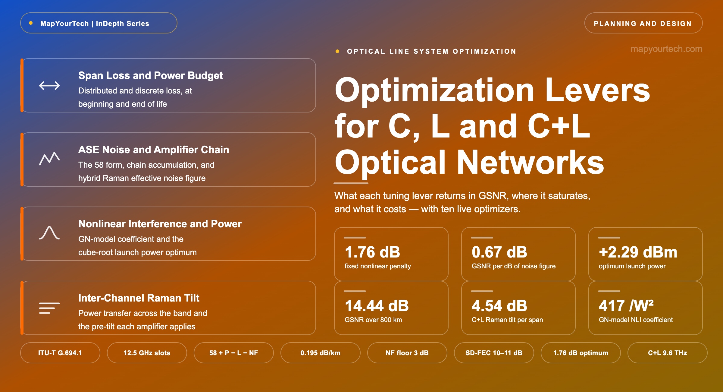
Optimization Levers for C, L and C+L Optical Networks
Every formula in optical line design, paired with a live optimizer: what each tuning lever returns in GSNR, where it saturates, and what it costs.
What you can measure, you can improve.
1. Introduction
A 400 Gb/s channel that misses its margin check by 1.5 dB has at least six ways out, and they differ in cost by four orders of magnitude. Retuning the per-channel launch power costs an afternoon on a network management terminal. Cleaning four connector pairs costs a technician visit. Swapping every amplifier on the route for a lower-noise variant costs a hardware programme. Adding distributed Raman gain costs pump hardware, power and a new correlated failure mode. Removing two spans costs civil work. Stepping the line rate down to 350 Gb/s costs 50 Gb/s of revenue-bearing capacity, forever. All six close the same 1.5 dB gap. Choosing between them is the work, and it depends on knowing what each lever returns before anyone is dispatched.
That knowledge exists, and it is not mysterious. Every quantity a planner adjusts on an optical line system appears in one of about a dozen closed-form relations, and the derivative of received Generalized Signal-to-Noise Ratio (GSNR) with respect to each of them can be written down. The problem is that those relations are usually met one at a time, in isolation, inside a planning tool that returns a single number and no sensitivity. An engineer learns that lowering amplifier noise figure improves Optical Signal-to-Noise Ratio (OSNR) by an equal amount, which is true in a linear link and wrong by a third in a link running at its nonlinear optimum. An engineer learns that raising launch power raises OSNR, which is true until nonlinear interference takes over and the same action lowers GSNR. The relations interact, and the interactions are where the design decisions live.
This article is built around that gap. It sets out the working formula set for C-band, L-band and C+L transmission design, and beneath each formula it places a live Formula Sandbox: a calculator with sliders on every input, a curve that redraws as the inputs move, and a result band that says whether the current setting passes. The defaults in every sandbox reproduce one worked reference link, so the numbers in the prose and the numbers on the screen are the same numbers. Change a slider and the article's example becomes yours.
1.1 Scope and the Reference Link
The reference link used throughout is deliberately ordinary: ten spans of 80 km G.652.D fiber, 0.195 dB/km attenuation, 0.25 splices per kilometre at 0.10 dB each, four connector pairs at 0.35 dB, giving 19.0 dB of span loss at beginning of life and 22.0 dB after a 3 dB ageing and repair allowance [computed from the loss model in Section 6]. Erbium-doped fiber amplifiers with a 5.0 dB noise figure recover each span. The channel plan is a 400 Gb/s carrier at 69.4 GBd with 15% forward error correction overhead in an 87.5 GHz flexible-grid slot. On that link the closed-form Gaussian noise model puts the optimum launch power at +2.29 dBm per channel and the delivered GSNR at 14.44 dB, against a requirement of 12.62 dB, leaving 1.82 dB before system and filter margin is taken out [all values computed from the model set in Section 5]. The link is therefore realistic in the least comfortable sense: it works, and it does not have much to spare.
Three bands are in scope. The C-band occupies 1530–1565 nm, about 4.8 THz of usable spectrum on a conventional erbium amplifier. The L-band occupies 1565–1625 nm and adds roughly 4.8 THz more, though at higher fiber attenuation and higher amplifier noise figure. Operating both together as C+L roughly doubles fiber capacity without new cable, and introduces one mechanism that a C-band-only design never has to model: inter-channel stimulated Raman scattering (ISRS), which transfers power from the shorter-wavelength half of the spectrum into the longer. Every section that follows carries the C+L case explicitly rather than treating it as a footnote, because the tilt this transfer produces changes the span loss that every channel sees, in both bands, whenever the channel plan changes.
1.2 Requirements of a Usable Optimizer
A useful optimizer answers three questions rather than one. First, what is the value now: the delivered GSNR, the margin against the requirement, and which noise term is binding. Second, what is the local derivative: how much GSNR one decibel of each lever returns, at the current operating point, after every coupled quantity has responded. Third, what is the reachable range: whether the lever has enough travel to close the gap at all, or whether it saturates first.
The second question is the one that separates a model from a lookup table. Launch power couples almost every other parameter together, because the optimum launch power is itself a function of span loss, noise figure, span count, baud rate and occupied bandwidth. Improve the noise figure by 1 dB and the amplified spontaneous emission (ASE) floor drops by 1 dB, but the optimum launch power also rises by a third of a decibel, which raises nonlinear interference, and the net GSNR return settles at 0.67 dB [derived in Section 8]. That two-thirds factor is not a correction term; it is the answer, and a design conversation that uses 1.0 dB instead will over-promise on every amplifier upgrade it recommends.
The third question is the one that stops wasted work. Raman on-off gain improves effective noise figure steeply up to about 8 dB of gain and then flattens: going from 10 dB to 15 dB of on-off gain buys 0.69 dB of effective noise figure while roughly doubling pump power [computed from the Friis cascade in Section 7]. Occupied bandwidth has a similar shape in the other direction. Knowing where a lever runs out is worth as much as knowing its slope.
1.3 Structure
Sections 2 to 4 establish the frame: how the field arrived at the current design rules, how GSNR partitions into independent noise terms, and how a C+L line system is physically arranged. Section 5 collects the complete formula set in one table so it can be used as a reference without reading the derivations. Sections 6 to 11 take one formula group each — span loss, amplifier noise, nonlinear interference, Raman tilt, transceiver requirement, and reach against margin — and pair each with its sandbox and its lever table. Sections 12 and 13 apply the whole set to deployment cases and rank the levers against each other. Sections 14 and 15 mark the boundaries of the closed-form approach and the direction automated optimization is taking. Every number in the article is labelled with its evidence class, because a figure without one reads as marketing.
Takeaway: The formula set for optical line design is small and closed-form, but the parameters are coupled through launch power. Any lever evaluated without re-optimizing power returns the wrong number, usually by a third.
2. Historical Development of Optical Design Rules
The 58 form for per-span OSNR predates coherent detection by more than a decade and still sets the scale of every amplified link built today. Written as OSNR = 58 + Pch − Lspan − NF for a chain in which each amplifier exactly recovers its preceding span loss, it contains a constant, 58, that is nothing more than −10·log10(hν·Δνr) evaluated at 193.4 THz in a 0.1 nm reference bandwidth, which is 12.5 GHz [standard-specified reference bandwidth per ITU-T G.697]. The amplifier gain does not appear because it cancels. That cancellation is the single most common source of arithmetic error in the field: writing the per-span OSNR as P + G − L − NF returns a number near zero and condemns a healthy link. The OSNR fundamentals treatment on this site works through the correct anchoring in detail.
2.1 Dispersion-Managed Design and Its Assumptions
Systems built before coherent receivers managed chromatic dispersion optically, with dispersion compensation modules inserted at amplifier sites. Those designs had a hard ceiling on launch power that came from a different mechanism than the one that binds today. With low accumulated dispersion between spans, four-wave mixing was efficient and channel spacings had to stay wide or dispersion had to be kept deliberately non-zero. Design rules from that era carry per-channel power thresholds tied to fiber type, and an accumulated-power threshold summed along the path rather than a per-span optimum. Those rules were correct for their systems and do not transfer: with dispersion compensation removed, the nonlinear penalty stops behaving like a threshold and starts behaving like additive noise.
2.2 The Gaussian Noise Model and the Additive-Noise Picture
Coherent receivers made optical dispersion compensation unnecessary, and uncompensated propagation changed what nonlinearity does to a signal. In a link with high local dispersion and no inline compensation, adjacent channels walk off each other quickly, the interfering field statistics approach Gaussian within the first spans, and the resulting distortion can be treated as an additive noise term rather than a deterministic distortion. That is the content of the Gaussian Noise (GN) model, and it is what makes a single scalar — GSNR — adequate to predict performance across formats.
The model rests on four assumptions, and each has a boundary. The signal must be spectrally broad and flat relative to the Kerr correlation bandwidth. Local dispersion must be high enough that inter-channel walk-off is short against the span. The link must stay inside the perturbative range, which holds up to roughly 2 dBm per channel on standard single-mode fiber. And nonlinear interference must accumulate incoherently across spans, so that powers add. Where those hold, GN predictions have been validated within about 1 dB for more than 90% of samples in multi-vendor testbeds [measured]. Where they do not, the corrections are known: the enhanced Gaussian noise model removes the constellation-dependent over-estimate that the Gaussian assumption produces for square quadrature amplitude modulation formats, and the ISRS-GN and generalized GN models extend the treatment to C+L and Raman-amplified links where stimulated Raman scattering tilts power across the band. Published closed-form ISRS-GN approximations match numerically integrated models to about 0.1 dB in nonlinear interference power [measured against split-step simulation].
Read the Full Analysis with Premium
The remaining 88% of this article — the design numbers, trade-offs and field guidance — is part of MapYourTech Premium, along with the full premium library, courses and professional tools.
You May Also Like

-
Premium
-
August 18, 2026
-
Free
-
August 18, 2026
-
Free
-
August 18, 2026