BOL and EOL Margin Design for OSNR, GOSNR and Q
How the beginning-of-life and end-of-life operating points of an amplified link are derived, where each aging allowance enters the noise budget, and what separates a defensible margin from a padded one.
The best network design is one that anticipates tomorrow's needs.
What You Will Learn
- Define BOL and EOL as the two evaluation points of one link, and name what changes between them: span loss, linear penalties and transceiver aging.
- Place the four margin classes at their exact insertion points in a planning model: span-loss aging, linear penalties, transceiver aging and model uncertainty.
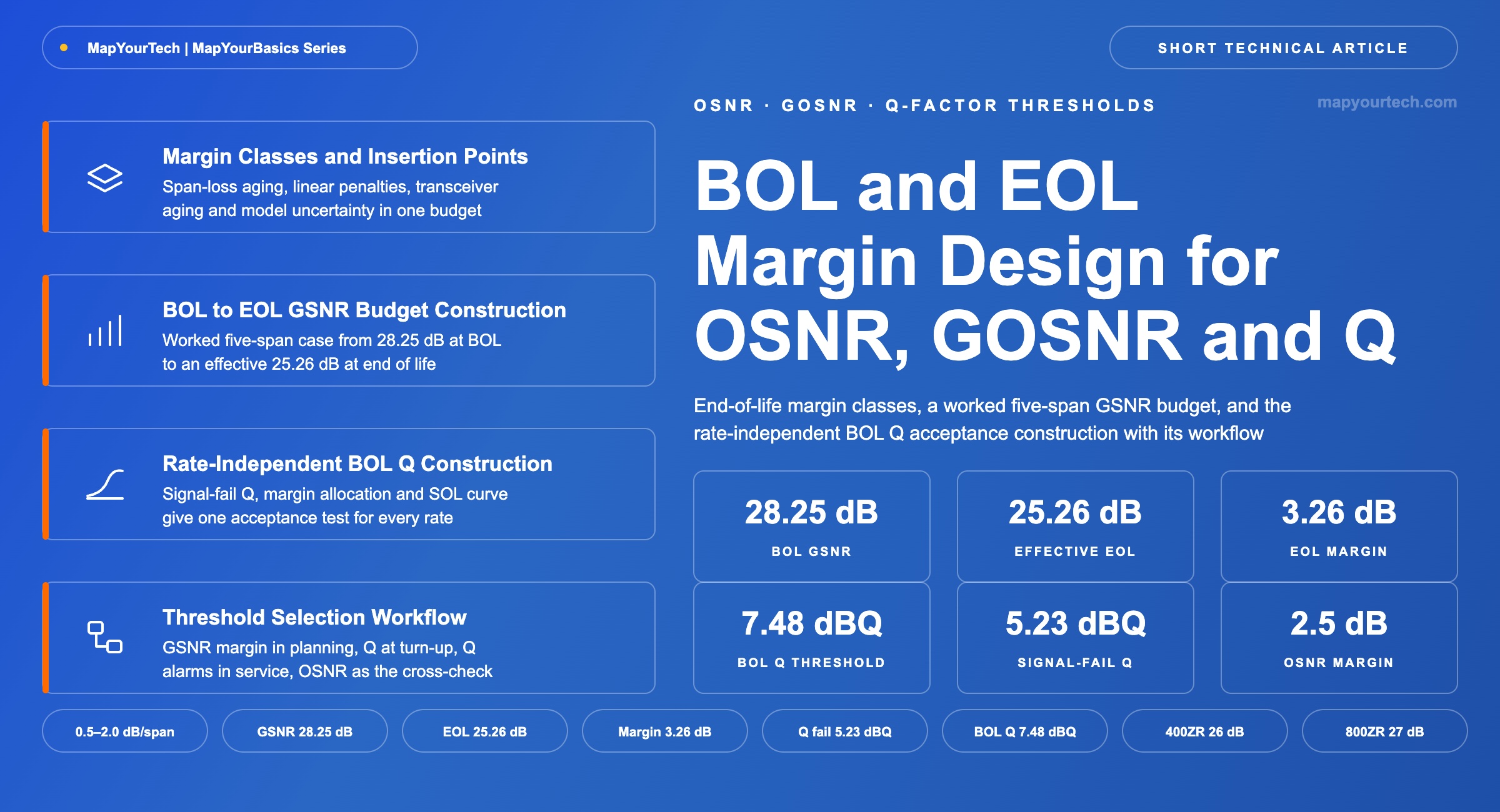
- Build a BOL-to-EOL GSNR budget on a worked five-span case, from 28.25 dB at commissioning to an effective 25.26 dB at end of life.
- Quantify aging sensitivity: how a 0 to 2.0 dB per-span allowance moves the EOL margin from 3.95 dB down to 2.52 dB on the same path.
- Anchor designs to standard-specified receiver OSNR: OpenZR+ 24, 400ZR 26 and 800ZR 27 dB/0.1 nm.
- Construct the rate-independent BOL Q acceptance threshold in three steps: 5.23 dBQ at signal fail, 2.5 dB of OSNR margin, 7.48 dBQ on the SOL curve.
- Convert pre-FEC BER to Q-factor with one relation that contains no rate term, so a single table serves 100G through 800G.
- Select the right quantity at each stage: GSNR margin in planning, Q at turn-up, Q alarm thresholds in service, with OSNR as the localization cross-check.
1. Introduction
A planning tool that reports 28.25 dB of generalized signal-to-noise ratio (GSNR) on a five-span path has told you what the link does on the day it is commissioned. It has not told you whether the link still carries traffic after three fiber repairs, a connector re-termination and eight years of slow attenuation drift. Those are two different numbers, and the gap between them is the design margin an operator commits to at the moment the route is signed off.
Beginning-of-life (BOL) and end-of-life (EOL) are the two evaluation points of that budget. ITU-T G-series system design has specified optical parameters at end-of-life since the single-channel era: minimum receiver sensitivity in the ITU-T optical interface Recommendations is defined for the worst case and end-of-life condition, with connector degradation, measurement tolerance and aging effects all inside the definition. Coherent systems moved the governed quantity from received power to GSNR, but the two-point discipline did not change.
This article sets out what BOL and EOL mean for optical signal-to-noise ratio (OSNR) and generalized OSNR (GOSNR), which margin classes belong to each, where each one enters a Gaussian Noise (GN) model calculation, and how to build the budget for a concrete five-span path. It closes with the standard-specified receiver OSNR requirements the resulting EOL figure is compared against.
2. Beginning-of-Life and End-of-Life Definitions
BOL is the modelled performance of the path with every component at its commissioning value: measured span loss from the as-built optical time-domain reflectometer (OTDR) traces, amplifier noise figure at the type-tested value, connectors freshly cleaned, and the transceiver at the top of its manufacturing distribution. EOL is the same path evaluated with every one of those quantities displaced to the worst value the operator is prepared to accept over the service life of the system. Neither is a measurement; both are model outputs from the same physics with different inputs.
Three properties separate them, and each one changes how the number should be used.
- BOL is falsifiable, EOL is not. A commissioning test measures BOL directly and the model can be corrected against it. EOL is a prediction about a plant state that has not occurred, so its accuracy depends entirely on the allowances chosen. The commissioning record is the only calibration anchor the EOL figure ever gets.
- The two points move different noise terms. Added span loss raises the amplifier gain needed to close the span, which lowers the input power to the next amplifier and increases accumulated amplified spontaneous emission (ASE). It does not change the nonlinear interference (NLI) generated in the fiber, because launch power per span is held at its target. GSNR therefore degrades by less than OSNR does.
- Only EOL governs the feasibility decision. A lightpath that closes at BOL and fails at EOL is not a feasible lightpath. The BOL number is reported for commissioning verification, not for route selection.
The reference bandwidth convention applies to both points without exception. OSNR and GSNR are quoted in the 0.1 nm reference bandwidth, about 12.5 GHz near 1550 nm, and compared against transceiver thresholds stated in the same bandwidth. Mixing a 0.1 nm path figure with a symbol-rate receiver signal-to-noise ratio produces an error of several decibels; the GOSNR and OSNR composition treatment works through the conversion, and the OSNR fundamentals primer covers the underlying noise accounting.
Takeaway: Report BOL and EOL as a pair on every design record. BOL is what commissioning will confirm; EOL is what the service commitment rests on, and only EOL decides feasibility.
3. Margin Classes and Planning-Model Insertion Points
An EOL allowance is not a single number applied at the end of the calculation. It resolves into four classes that enter the model at different places and behave differently under changes to launch power, span count and modulation format. Collapsing them into one lump sum is what produces budgets that are simultaneously too conservative on short paths and too optimistic on long ones.
The open-source GN-model planning library GNPy exposes three of the four as named parameters, which makes it a convenient reference for naming the insertion points. Its span-level EOL parameter is documented as fiber span loss aging, and the tool adds its value to the fiber output connector so that design and feasibility are performed with span loss plus that allowance. Transceiver-side aging is carried by sys_margins, documented as added margin on the minimum required transceiver OSNR. Linear transmission penalties are carried by a penalties list indexed by chromatic dispersion (CD), polarization mode dispersion (PMD) and polarization dependent loss (PDL), and the accumulated penalties are subtracted from the path GSNR before the comparison with the minimum required OSNR. These are tool-specified mechanisms, and every commercial planner implements equivalents under its own names.
| Margin class | Physical cause | Insertion point in the model | Typical allocation | Evidence class |
|---|---|---|---|---|
| Span-loss aging and repair | Attenuation drift, added splices and slack loops from cable repairs, connector re-termination | Loss added per span at the fiber output connector, before amplifier gain is set | 0.5–2.0 dB per span | Planning practice |
| Linear transmission penalties | Accumulated CD, PMD and PDL evaluated against the transceiver tolerance curve | Subtracted from path GSNR before the threshold comparison | 0.3–1.0 dB per path | Tool-specified mechanism |
| Transceiver aging | Laser and receiver drift, module replacement across a vendor population | Added to the minimum required transceiver OSNR | 0.5–1.5 dB per path | Planning practice |
| Model uncertainty | GN-model error, amplifier gain ripple, uncharacterised wavelength selective switch (WSS) filtering | Threshold offset applied by the planning tool | 0.7–1.0 dB per path | Vendor planning-tool convention |
| Channel-load change | Full-fill stimulated Raman scattering tilt and ASE loading at EOL against partial fill at turn-up | Re-run of the design at full spectral load | 0.92 dB and 1.46 dB recommended in one open line system study | Measured |
The last row is worth separating from the others because it is measured rather than assumed. An experimental characterisation of optical spectrum as a service on a terrestrial brownfield system, carried out on the Open Ireland testbed and verified on the HEAnet production network, recommends a minimum of 0.92 dB of service margin to absorb the effect of enabling neighbouring channels and 1.46 dB to absorb end-of-life channel loads, with a further 0.6 dB of GSNR margin for probing accuracy. Those are measured allocations for a specific system class, not universal constants, but they set a useful floor: a design that allocates less than a decibel for the difference between a lightly loaded turn-up spectrum and a fully loaded EOL spectrum is allocating less than a published measurement supports.
ITU-T system design guidance states the same principle for the loss budget without fixing a number, requiring that a suitable margin be allocated for future modifications of cable configurations, covering additional splices, extra cable lengths, aging effects and temperature variations. The concatenated link attenuation it is applied to is the sum of the fiber attenuation coefficient over the link length, the mean splice loss times the splice count, and the mean connector loss times the connector count.
Allocate span-loss aging per span and threshold-side allowances per path. An allowance applied at the wrong scope changes the answer: a 1.0 dB per-span figure applied once to a ten-span route understates EOL loss by 9 dB, and a per-path figure applied to every span overstates it by the same arithmetic.
Takeaway: Name each margin class, its scope and its evidence class in the design record. A budget line labelled only "margin: 3 dB" cannot be audited, re-used on a different route, or reduced when better data arrives.
4. GSNR Budget Construction from BOL to EOL
The BOL calculation starts from the ASE cascade relation for a chain of identical spans, where the 58 dB constant is the magnitude of the quantum noise floor over the 12.5 GHz reference bandwidth at 193.4 THz.
ASE-only OSNR for N identical spans
OSNR_ASE (dB) = P_ch − NF − L_span + 58 − 10*log10(N)Where:
P_ch — per-channel launch power into each span, dBm (typical −3 to +2 dBm)
NF — amplifier noise figure, dB (typical 4.5–6.5 dB for a C-band EDFA)
L_span — span loss including connectors and the EOL aging allowance, dB (typical 14–25 dB)
N — number of identical amplified spans in the path
Nonlinear interference is added in the same reference bandwidth by the reciprocal composition rule, because ASE and NLI are treated as independent additive Gaussian contributions and their powers add directly.
Composition of ASE and nonlinear interference
1 / GSNR = 1 / OSNR_ASE + 1 / SNR_NLI          (linear ratios)

GSNR (dB) = −10*log10( 10^(−OSNR_ASE/10) + 10^(−SNR_NLI/10) )
Where:
SNR_NLI — the NLI-only ratio, per-channel power divided by accumulated nonlinear interference power, dB
GSNR — generalized signal-to-noise ratio at the 0.1 nm reference bandwidth, dB
The EOL feasibility test then applies the four margin classes at their correct insertion points and compares the result against the transceiver threshold.
End-of-life margin
GSNR_EOL = GSNR( L_span + dL_EOL )

M_EOL = GSNR_EOL − P_lin − ( OSNR_req + S_marg + U_model )
Where:
dL_EOL — per-span aging and repair allowance, dB (typical 0.5–2.0 dB)
P_lin — accumulated CD, PMD and PDL penalty on the path, dB
OSNR_req — minimum required receiver OSNR at 0.1 nm for the selected mode, dB
S_marg — transceiver aging allowance added to the requirement, dB
U_model — planning-tool model uncertainty offset, dB
M_EOL — end-of-life margin; the lightpath is feasible when M_EOL is positive
Practical Example — five-span 400 km path at 64 GBd
Take five identical 80 km G.652.D spans at 0.20 dB/km, giving 16.00 dB of span loss at commissioning, each followed by an erbium-doped fiber amplifier (EDFA) with a 5.00 dB noise figure. The channel is 64 GBd dual-polarization 16QAM (DP-16QAM) launched at 0 dBm. The ASE-only figure is 0 − 5.00 − 16.00 + 58 − 6.99 = 30.01 dB. With the NLI-only ratio at 33.02 dB for this path, the composition rule gives a BOL GSNR of 28.25 dB, sitting the expected 1.76 dB below the ASE-only value because 0 dBm is the optimum launch power here.
Now apply a 1.00 dB per-span aging and repair allowance. Span loss becomes 17.00 dB, the ASE-only figure falls to 29.01 dB, and SNR_NLI is unchanged at 33.02 dB because launch power per span is still 0 dBm. The composition rule returns 27.56 dB. The path lost 1.00 dB of OSNR and only 0.69 dB of GSNR — a direct consequence of NLI holding constant while ASE grows. Adding 0.50 dB of linear penalties, 1.00 dB of transceiver aging and 0.80 dB of model uncertainty leaves an effective EOL GSNR of 25.26 dB, and against a required OSNR of 22.00 dB (a representative figure inside the widely published 21–23 dB transceiver-class range for 400G DP-16QAM, not a single vendor specification) the EOL margin is 3.26 dB. The cascaded-span OSNR relation generalises the 58 dB constant to unequal spans, and the EDFA noise figure treatment covers the ASE half of this budget.
| Step | Quantity | Value (dB) | Running GSNR (dB) |
|---|---|---|---|
| 1 | BOL GSNR at commissioning | 28.25 | 28.25 |
| 2 | Span-loss aging, 1.00 dB per span | −0.69 | 27.56 |
| 3 | Linear penalties (CD, PMD, PDL) | −0.50 | 27.06 |
| 4 | Transceiver aging allowance | −1.00 | 26.06 |
| 5 | Model uncertainty allowance | −0.80 | 25.26 |
| 6 | Required OSNR, 400G DP-16QAM class | 22.00 | — |
| 7 | EOL margin | 3.26 | — |
Takeaway: Span-loss aging costs less GSNR than it costs OSNR, because nonlinear interference does not follow span loss when launch power is held at target. A budget that applies the aging allowance directly to GSNR overstates the loss by roughly 0.3 dB per decibel on a path at optimum launch power.
5. Sensitivity to Per-Span Aging Allowance
The per-span allowance is the single input with the largest influence on the EOL result, and it is the one with the weakest evidence behind it in most design records. Sweeping it across the range operators commonly use shows how much reach the choice costs. Holding the threshold-side allowances constant at their combined 2.30 dB, the effective EOL GSNR for the five-span path falls from 25.95 dB with no aging allowance to 24.52 dB at 2.00 dB per span — a total swing of 1.43 dB across the full range of the input.
| Allowance (dB/span) | Span loss (dB) | ASE-only OSNR (dB) | Path GSNR (dB) | Effective EOL GSNR (dB) | EOL margin (dB) |
|---|---|---|---|---|---|
| 0.0 | 16.00 | 30.01 | 28.25 | 25.95 | 3.95 |
| 0.5 | 16.50 | 29.51 | 27.91 | 25.61 | 3.61 |
| 1.0 | 17.00 | 29.01 | 27.56 | 25.26 | 3.26 |
| 1.5 | 17.50 | 28.51 | 27.19 | 24.89 | 2.89 |
| 2.0 | 18.00 | 28.01 | 26.82 | 24.52 | 2.52 |
Two points follow from the shape of the curve. The sensitivity is mild on a five-span C-band path at optimum launch power, so a conservative allowance costs little; on a twenty-span path with the same per-span figure, the ASE term grows four times faster and the same choice decides whether 16QAM or QPSK carries the service. And because the deduction acts on ASE alone, a path that is already nonlinearity-limited absorbs aging better than one that is ASE-limited — the reciprocal composition means the larger noise term dominates and the smaller one moves the result very little. The GN model treatment develops the underlying scaling, and the link engineering formula reference collects the related expressions.
Takeaway: Sweep the per-span allowance rather than fixing it. On short ASE-rich paths the choice is nearly free; on long paths it selects the modulation format, and that is where the evidence behind the number has to be strongest.
The workbench below runs the same budget live. Every default reproduces the worked case of Table 2, the chart redraws the aging sweep of Figure 2 for any path, and the second panel carries the Q-threshold construction of Section 7 with the same required-OSNR anchor.
At the defaults the workbench reproduces the worked case: BOL GSNR 28.25 dB, effective EOL GSNR 25.26 dB, EOL margin 3.26 dB, BOL Q threshold 7.48 dBQ.
6. Receiver Threshold Reference and Verification Practice
The EOL figure is only as useful as the threshold it is compared against. For the pluggable coherent classes the requirement is standard-specified rather than inferred, and each interface pairs the modulation with a defined forward error correction (FEC) scheme, which removes one source of uncertainty from the budget entirely.
| Interface | Modulation | Required Rx OSNR (dB/0.1 nm) | Specifying body |
|---|---|---|---|
| 400ZR | DP-16QAM with concatenated FEC | ≤ 26 | OIF 400ZR Implementation Agreement |
| OpenZR+ | DP-16QAM with open FEC | 24 | OpenZR+ Multi-Source Agreement |
| 800ZR | DP-16QAM with open FEC | ≤ 27 | OIF 800ZR Implementation Agreement |
Interoperability testing shows how much of that requirement a real module population consumes. Across the vendor pairings measured at recent OIF plugfests, most combinations met the 400ZR requirement of 26 dB/0.1 nm, with a small number of pairs measuring between 26.2 and 26.4 dB/0.1 nm; the 800ZR results followed the same pattern against the 27 dB/0.1 nm limit. Those are measured values from multi-vendor test events. The practical consequence for an EOL budget is that a design sized against the specification limit already absorbs the observed spread, while a design sized against a single vendor's typical figure does not.
Verification closes the loop between the two evaluation points. The BOL figure is confirmed at turn-up by comparing the transceiver's reported signal-to-noise ratio and the optical channel monitor spectrum against the model output, which is the subject of channel monitoring with OCM and OSA. The EOL figure cannot be verified at turn-up, so what is tracked instead is the rate at which the real plant consumes the allowance: span loss trended from the optical supervisory channel and periodic OTDR runs, amplifier gain and noise figure trended from telemetry, and the difference between predicted and measured GSNR trended over time. A model that tracked within a decibel at commissioning can drift by two to three decibels after a few years of repairs and card swaps, which is the argument for scheduled recalibration rather than one-time design; digital twin calibration loops and in-house multivendor planning practice cover the operational side, and the OSNR against GOSNR simulator lets the budget above be re-run against different span and amplifier inputs.
Record the measured BOL GSNR against the predicted BOL GSNR at commissioning, and treat the difference as the starting error of the EOL prediction. An unrecorded commissioning delta means the EOL margin has an unknown offset for the whole life of the system.
Takeaway: Size the budget against the specification limit, not a typical datasheet figure, and trend allowance consumption from live telemetry. The EOL number earns its authority from the measurement programme behind it, not from the size of the allowance.
7. BOL Threshold Construction from the Q-Versus-OSNR Curve
A commissioning engineer does not read GSNR off a transceiver. The module reports pre-FEC bit error ratio (BER), and the acceptance test is a Q-factor threshold. Converting the EOL budget of Section 4 into a number a field team can act on at turn-up is a three-point construction on a pair of Q-versus-OSNR curves: the start-of-life typical curve and the end-of-life worst-case curve. Start-of-life and beginning-of-life name the same evaluation point; vendor curve sets label it SOL, planning documents label it BOL.
The construction runs backwards from the failure condition, which is why it produces a threshold that already contains the whole margin stack:
- Read the required OSNR. On the end-of-life worst-case curve, find the OSNR at the signal-fail Q threshold. That OSNR is the required OSNR, written rOSNR, and it is the zero point of the normalized axis. The EOL curve already carries propagation penalties, aging, and worst-case temperature and manufacturing spread, so this point needs no further deduction.
- Add the OSNR margin allocation. Move right along the axis by the operational margin the design commits to. One vendor deployment convention allocates 2.0 dB for propagation and repair effects plus 0.5 dB for transients, giving 2.5 dB in total. The sum is the required BOL OSNR.
- Read the acceptance threshold. At that OSNR, read up to the start-of-life typical curve. The Q value there is the BOL Q threshold used for deployment acceptance. A wavelength that turns up above it has the full margin stack in hand; one that turns up below it does not, whatever its measured OSNR says.
The reason a single construction serves every line rate is that the two axes carry different kinds of dependence. Line rate, modulation format and baud rate set where the curve sits on the absolute OSNR axis, so normalizing the horizontal axis to the interface's own rOSNR removes that offset. The vertical axis is already rate-independent: Q follows from pre-FEC BER through a relation that contains no rate term at all, and the signal-fail and signal-degrade thresholds are properties of the FEC scheme rather than the line rate. The two datum lines drawn for one FEC therefore serve every rate that FEC carries; a family running a different FEC redraws them at its own thresholds and the construction itself is unchanged.
Pre-FEC BER to Q-factor, rate-independent
Q² (dB) = 20*log10( sqrt(2) * erfcinv( 2 * BER ) )

BER = 0.5 * erfc( 10^(Q²/20) / sqrt(2) )        (inverse form)
Where:
BER — pre-FEC bit error ratio reported by the receiver; the signal-fail threshold is a property of the FEC scheme (Table 5)
erfcinv — inverse complementary error function; erfc — complementary error function
Q² — Q-factor expressed in dB, the form transceivers and planning tools report
The relation contains no baud rate, modulation or FEC term, so one conversion table serves every interface.
| Pre-FEC BER | Q² (dB) | Margin to fail (dBQ) | Common use of this point |
|---|---|---|---|
| 1.0×10⁻² | 7.33 | 2.11 | Healthy operating point on a commissioned wavelength |
| 2.0×10⁻² | 6.25 | 1.03 | Early warning band on a degrading path |
| 2.66×10⁻² | 5.73 | 0.50 | Signal-degrade alarm in one vendor convention |
| 3.0×10⁻² | 5.49 | 0.26 | Signal-fail threshold of an earlier coherent generation |
| 3.4×10⁻² | 5.23 | 0.00 | Signal-fail threshold of the Figure 3 curve set; rOSNR anchor |
| 4.0×10⁻² | 4.86 | −0.36 | Past the correction limit; post-FEC errors present |
The margin column is anchored to the 3.4×10⁻² signal-fail threshold of the Figure 3 curve set. An interface running the 400ZR concatenated FEC instead reaches signal fail near a pre-FEC BER of 1.22×10⁻², a standard-specified threshold from the OIF 400ZR Implementation Agreement that converts to a signal-fail Q² near 7.0 dB, and its margin column re-anchors there. The conversion itself never changes; only the anchor row moves with the FEC.
Applying the construction to the standard-specified thresholds of Section 6 gives the BOL OSNR each interface has to reach at turn-up. The margin allocation is the same 2.5 dB in every row because it covers path effects rather than transceiver behaviour, which is what makes the recipe portable across rates.
| Interface | rOSNR at signal fail (dB/0.1 nm) | Margin allocation (dB) | Required BOL OSNR (dB/0.1 nm) |
|---|---|---|---|
| OpenZR+ | 24.0 | 2.5 | 26.5 |
| 400ZR | 26.0 | 2.5 | 28.5 |
| 800ZR | 27.0 | 2.5 | 29.5 |
Set the turn-up acceptance test on Q, not on OSNR. A wavelength can measure the required BOL OSNR on the optical spectrum analyser and still sit below the BOL Q threshold when transceiver spread or an unmodelled filtering penalty is present; the Q reading catches that case and the OSNR reading does not.
Takeaway: Build the acceptance threshold from the failure point outwards: signal-fail Q on the EOL curve gives rOSNR, the margin allocation gives the required BOL OSNR, and the SOL curve at that OSNR gives the BOL Q a field team tests against. Normalizing the OSNR axis to rOSNR makes one construction cover every rate on the network.
The explorer below makes the construction of Figure 3 draggable. The margin handle moves point 2 and the acceptance threshold with it, the amber operating point rides the aged curve, and the interface chips load the standard-specified anchors of Table 6.
At the defaults the explorer reads the reference construction: 5.23 dBQ at signal fail, a 2.5 dB OSNR margin, and a 7.48 dBQ BOL acceptance threshold.
8. Threshold Selection and Verification Workflow
The preceding sections produce three different threshold quantities: a GSNR margin for planning, a Q threshold for turn-up acceptance, and a pair of Q alarm thresholds for operation. Each belongs to one stage of a wavelength's life, and Figure 4 places them in the order a wavelength meets them. Planning tests the effective end-of-life GSNR against the required OSNR; a margin of at least 0 dB releases the design, and anything less routes back through span-loss reduction, an added amplifier site, or a lower-order format. Turn-up tests measured pre-FEC Q against the BOL Q threshold of Section 7. The OSNR reading taken at the same time is not the acceptance test; it is the localization tool. A wavelength short on Q but meeting the required BOL OSNR points at the transceiver or the filtering path, while one short on both points at span loss, amplifier gain, or tilt. In service, the same Q scale carries the alarm thresholds: signal degrade means the committed margin is spent, and signal fail means post-FEC errors are present.
Table 7 compresses the workflow into the quantity, threshold source, and action per stage, with the worked reference values carried through from the budget and the curve construction.
| Stage | Quantity under test | Threshold source | Result and action |
|---|---|---|---|
| Planning | EOL GSNR margin | Effective EOL GSNR minus the required OSNR | Proceed at 0 dB or more; redesign otherwise. Reference case: 3.26 dB. |
| Turn-up acceptance | Pre-FEC Q | BOL Q from the curve construction | Accept at or above the threshold. This curve set: 7.48 dBQ. |
| Turn-up cross-check | OSNR at 0.1 nm | Required BOL OSNR, rOSNR plus the margin allocation | Localizes a Q shortfall to the line or the transceiver. Reference case: 24.50 dB. |
| Operation, first alarm | Pre-FEC Q | Signal-degrade threshold | At 5.73 dBQ in one vendor convention the committed margin is spent; schedule the intervention. |
| Operation, service limit | Pre-FEC Q | Signal-fail threshold | At 5.23 dBQ post-FEC errors are present; restore OSNR or protection-switch, then requalify. |
Takeaway: Test GSNR margin in planning, Q at turn-up, and Q against the alarm thresholds in service, and use the OSNR cross-check to localize a shortfall rather than to accept a wavelength. The redesign, remediation and requalification loops are the defined return paths when a test does not pass.
9. Summary
BOL and EOL are the same GN-model calculation evaluated with commissioning inputs and worst-accepted-case inputs. Four margin classes separate them, and each enters at a different point: span-loss aging as added loss per span before amplifier gain is set, linear CD, PMD and PDL penalties as a subtraction from path GSNR, transceiver aging as an addition to the required OSNR, and model uncertainty as a threshold offset. Because span-loss aging acts on ASE alone while nonlinear interference stays fixed at constant launch power, GSNR degrades more slowly than OSNR does.
Quick reference values from the five-span 64 GBd example: 28.25 dB BOL GSNR; 25.26 dB effective EOL GSNR; 2.99 dB consumed across four margin classes; 3.26 dB EOL margin against a 22.00 dB requirement. Standard-specified receiver requirements are 26 dB/0.1 nm for 400ZR, 24 dB/0.1 nm for OpenZR+ and 27 dB/0.1 nm for 800ZR. Typical planning allocations are 0.5–2.0 dB per span for aging and repair, 0.3–1.0 dB for linear penalties, 0.5–1.5 dB for transceiver aging and 0.7–1.0 dB for model uncertainty.
The budget becomes a field-testable number through a three-point construction on the Q-versus-OSNR curve pair: signal-fail Q on the end-of-life worst-case curve fixes rOSNR, the OSNR margin allocation fixes the required BOL OSNR, and the start-of-life typical curve at that OSNR fixes the BOL Q acceptance threshold. Because Q follows from pre-FEC BER with no rate term, and because the horizontal axis can be normalized to each interface’s own rOSNR, one construction covers every line rate on the network. For the curve set in Figure 3 the chain runs 5.23 dBQ at the failure point, 2.5 dB of OSNR margin, and 7.48 dBQ as the acceptance threshold. In service the same Q scale carries the signal-degrade and signal-fail alarm thresholds, so one quantity spans acceptance and monitoring while the OSNR reading serves as the localization cross-check.
References
- ITU-T G-series Supplement 39 — Optical system design and engineering considerations, ITU-T Study Group 15.
- ITU-T G.697 — Optical monitoring for dense wavelength division multiplexing systems, ITU-T Study Group 15.
- OIF-400ZR — Implementation Agreement for a 400ZR Coherent Optical Interface, Optical Internetworking Forum.
- OIF-800ZR — 800ZR Implementation Agreement, Optical Internetworking Forum.
- OpenZR+ Multi-Source Agreement — Multi-Vendor 400G Coherent Optical Transceiver White Paper, OpenZR+ MSA Group.
- Telecom Infra Project OOPT/PSE — GNPy: Optical Route Planning Library Based on a Gaussian Noise Model, Telecom Infra Project.
- K. Kaeval et al., Employing Channel Probing to Derive End-of-Life Service Margins for Optical Spectrum Services, Journal of Optical Communications and Networking.
- Sanjay Yadav, "Optical Network Communications: An Engineer's Perspective" — Bridge the Gap Between Theory and Practice in Optical Networking.
Related Articles on MapYourTech