Generic selectors
Exact matches only
Search in title
Search in content
Post Type Selectors
Articles
lp_course
lp_lesson
Back
HomeAnalysisLatency for Network Engineers: A Comprehensive Technical Guide
Latency for Network Engineers: A Comprehensive Technical Guide

Latency for Network Engineers: A Comprehensive Technical Guide

Last Updated: April 2, 2026
12 min read
112
Latency for Network Engineers: Comprehensive Technical Guide

Latency for Network Engineers: A Comprehensive Technical Guide

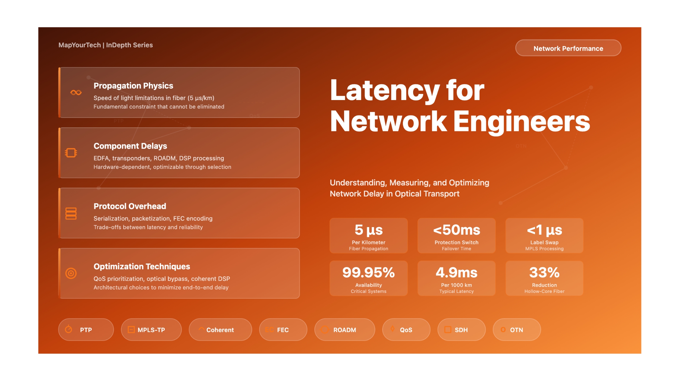
Understanding, Measuring, and Optimizing Network Delay in Modern Optical Transport Systems

Introduction

Latency has emerged as a critical performance parameter in modern optical networks, often matching or exceeding the importance of bandwidth in determining network quality. As applications become increasingly time-sensitive, from high-frequency trading requiring sub-microsecond response times to autonomous vehicles demanding millisecond-level precision, understanding and optimizing network latency has become essential for network engineers and architects.

This comprehensive guide examines latency from multiple perspectives: the fundamental physics governing signal propagation, the architectural choices that accumulate delay, the measurement techniques that quantify performance, and the optimization strategies that minimize end-to-end delay. Whether you are designing ultra-low-latency networks for financial services, implementing teleprotection systems for power utilities, or architecting next-generation cloud infrastructure, this article provides the technical foundation and practical insights needed to make informed engineering decisions.

The transition from bandwidth-centric to latency-aware network design represents a fundamental shift in telecommunications. While a 100 Gb/s link provides impressive throughput, if packets experience 50 ms of delay and 20 ms of jitter, the user experience degrades significantly. Conversely, a well-engineered 10 Gb/s network with consistent 2 ms latency can outperform higher-bandwidth alternatives for latency-sensitive applications. Understanding this trade-off space is central to modern network engineering.

Historical Evolution of Latency in Telecommunications

The evolution of telecommunications networks reflects a continuous balance between capacity, reach, and delay. In the early days of telegraph systems, latency was measured in minutes or hours as messages were manually relayed between stations. The introduction of telephone networks in the late 19th century reduced this to near real-time communication, with latency primarily determined by physical distance and the speed of electrical signals in copper wire.

The transition to digital telecommunications in the 1960s and 1970s introduced new sources of latency. Time Division Multiplexing systems like T1/E1 added framing delays and buffering requirements. The deployment of fiber optic networks in the 1980s promised reduced latency due to the speed of light in glass, but the reality proved more complex. While fiber offered lower propagation delay per kilometer compared to copper at equivalent distances, the optical-electrical-optical conversions required at each network node introduced additional delays.

Synchronous Digital Hierarchy and Synchronous Optical Network systems, standardized in the late 1980s, brought deterministic latency characteristics through their synchronous frame structure. A 125-microsecond frame period meant predictable, bounded delays at each multiplexing stage. However, the pointer adjustment mechanisms used to accommodate frequency variations could introduce occasional frame slips, creating small but measurable latency variations.

The shift to packet-based networks in the 1990s and 2000s fundamentally changed the latency landscape. Statistical multiplexing in IP/MPLS networks introduced variable queuing delays that could range from microseconds to milliseconds depending on network load. This variability, known as jitter, became a primary challenge for real-time applications. The development of Quality of Service mechanisms, including DiffServ and MPLS Traffic Engineering, aimed to provide bounded latency guarantees even in statistically multiplexed networks.

The emergence of coherent optical systems in the 2010s added another dimension to latency engineering. Digital Signal Processing in coherent transponders enables electronic dispersion compensation, eliminating the need for Dispersion Compensating Fiber that added 15-25% to the fiber propagation delay. However, the DSP itself introduces processing latency, typically ranging from tens to hundreds of nanoseconds depending on the algorithms employed.

Fundamental Principles of Network Latency

The Physics of Signal Propagation

At the most fundamental level, latency in optical networks is constrained by the speed of light. In a vacuum, light travels at exactly 299,792,458 meters per second. However, in optical fiber, light propagates more slowly due to the refractive index of the glass material. The effective group index of refraction determines the actual propagation velocity experienced by optical signals.

For standard single-mode fiber specified in ITU-T Recommendation G.652, the effective group index of refraction is approximately 1.4676 at 1310 nm and 1.4682 at 1550 nm. This yields a propagation velocity of approximately 204,200 km/s, or roughly two-thirds the speed of light in vacuum. The practical rule of thumb used by network engineers is that signal propagation in optical fiber introduces approximately 5 microseconds of delay per kilometer of distance.

Propagation Delay Calculation:

Delay = (Distance × neff) / c

Where:
  Distance = Fiber length in meters
  neff = Effective group index of refraction (dimensionless)
  c = Speed of light in vacuum = 299,792,458 m/s

Example: 1000 km fiber link at 1550 nm
Delay = (1,000,000 m × 1.4682) / 299,792,458 m/s
Delay  4,897 μs  4.9 ms

Rule of thumb: ~5 μs per km or ~5 ms per 1000 km

This propagation delay represents an absolute physical limit that cannot be reduced without changing the transmission medium. Various specialty fibers have been developed to minimize this delay. Hollow-core photonic crystal fibers, where light propagates primarily through air rather than glass, can reduce latency by up to 31% compared to conventional fiber. However, these specialty fibers typically exhibit higher attenuation (around 1.2-3.3 dB/km versus 0.2 dB/km for standard SMF at 1550 nm), limiting their practical deployment to high-value, latency-critical applications.

Serialization Delay: The Bandwidth-Latency Trade-off

Serialization delay represents the time required to transmit a data unit onto the physical link at a given bit rate. This component of latency is inversely proportional to link speed: higher bandwidth reduces serialization delay for a given packet size. Understanding this relationship is crucial for network design, particularly when dealing with variable packet sizes and mixed traffic types.

Serialization Delay Formula:

Delay = (Packet_Size × 8) / Link_Rate

Where:
  Packet_Size = Data unit size in bytes
  Link_Rate = Transmission rate in bits per second

Example: 1500-byte Ethernet frame at different speeds

At 100 Mb/s:  Delay = (1500 × 8) / 100,000,000 = 120 μs
At 1 Gb/s:    Delay = (1500 × 8) / 1,000,000,000 = 12 μs
At 10 Gb/s:   Delay = (1500 × 8) / 10,000,000,000 = 1.2 μs
At 100 Gb/s:  Delay = (1500 × 8) / 100,000,000,000 = 0.12 μs

Note: 10× bandwidth increase = 10× serialization delay reduction

The serialization delay becomes significant in lower-speed links or when transmitting large data units. For circuit emulation services carrying TDM traffic over packet networks, the packetization interval directly affects serialization delay. A 1 ms packetization interval at 2.048 Mb/s (E1 rate) yields 256 bytes per packet, introducing approximately 1 ms of serialization delay at the ingress point.

Figure 1: Components of End-to-End Network Latency
End-to-End Latency Breakdown in Optical Networks Propagation Delay ~5 μs/km × Distance Physics-limited, cannot be reduced Serialization Delay Packet_Size / Link_Rate Reduced by higher bandwidth Processing Delay 10-100 μs per node Hardware-dependent Queuing Delay Variable Load-dependent Typical Latency Values by Component Type Optical Fiber (SMF G.652) 4.897 μs/km @ 1550 nm, 4.895 μs/km @ 1310 nm EDFA (per amplifier) 50-200 ns (30m erbium-doped fiber ≈ 150 ns) Dispersion Compensating Fiber (DCF) 40-120 μs (20% of compensated fiber length) Fiber Bragg Grating (FBG) DCM 5-50 ns (much lower than DCF) ROADM / Optical Switch 5-10 μs per node Coherent Transponder (with DSP) Transparent: 2-30 ns, With FEC: 5-10 μs, With full DSP: up to 1 μs OEO Conversion (Regenerator) 10-100 μs depending on buffering requirements IP Router / L3 Switch (per hop) 25-100 μs for FIB lookup + forwarding Example: 2000 km Long-Haul Link Latency Calculation Given: 2000 km fiber, 25 EDFAs, 2 ROADMs, 40 km DCF, 2 coherent transponders Propagation (fiber): 2000 km × 5 μs/km = 10,000 μs = 10.0 ms Propagation (DCF): 40 km × 5.2 μs/km ≈ 208 μs = 0.208 ms EDFAs: 25 × 150 ns = 3,750 ns = 0.00375 ms ROADMs: 2 × 5 μs = 10 μs = 0.01 ms Transponders (with DSP): 2 × 0.5 μs = 1 μs = 0.001 ms Total One-Way Latency ≈ 10.22 ms (Propagation dominates at ~98% of total)

Key Takeaway: Latency Component Hierarchy

  • For long-haul links (>100 km), propagation delay dominates total latency, typically accounting for 95-98% of end-to-end delay
  • Serialization delay becomes negligible at modern speeds (≤1.2 μs for 1500-byte frames at 10 Gb/s)
  • Processing delays are cumulative across network nodes; a 10-hop network adds 250-1000 μs of processing latency alone
  • Queuing delay is the most variable component and requires careful QoS engineering to bound
  • Eliminating DCF through coherent DSP removes 15-25% of fiber-related latency at the cost of adding DSP processing delay
Premium Article — Free 21% Preview

Read the Full Analysis with Premium

The remaining 79% of this article — the design numbers, trade-offs and field guidance — is part of MapYourTech Premium, along with the full premium library, courses and professional tools.

Instant access · Cancel anytime · 48-hour trial available
Sanjay Yadav

Optical Communications & Network Automation Expert | Author of 3 Books for Optical Engineers | Founder, MapYourTech

Optical networking engineer with nearly two decades of experience across DWDM, OTN, coherent optics, submarine systems, and cloud infrastructure. Founder of MapYourTech.

Follow on LinkedIn

You May Also Like

15 min read 6 0 Like Connector Types and Their Loss Budgets: SC, LC, MPO Skip to main content MapYourTech...
  • Free
  • July 11, 2026
16 min read 6 0 Like Cooled vs Uncooled Lasers: The Pluggable Power Trade-off Skip to main content MapYourTech |...
  • Free
  • July 11, 2026
16 min read 7 0 Like Automation Blast Radius: Scoping What a Bad Intent Can Touch Skip to main content...
  • Free
  • July 11, 2026

Course Title

Course description and key highlights

Course Content

Course Details