Latency Impact in Each Networking Layer

1. Understanding the Components of Network Latency

Before examining latency at individual networking layers, we must understand the fundamental components that contribute to total end-to-end delay. Network latency is not a single value but rather the sum of multiple delay sources that accumulate as data traverses from source to destination.

1.1 Propagation Delay

Propagation delay represents the time required for electromagnetic or optical signals to physically travel through the transmission medium. This delay is fundamentally limited by the speed of light in the medium and is proportional to distance. In vacuum, light travels at approximately 299,792 km/s. However, in practical transmission media, signals propagate more slowly due to the refractive index of the material.

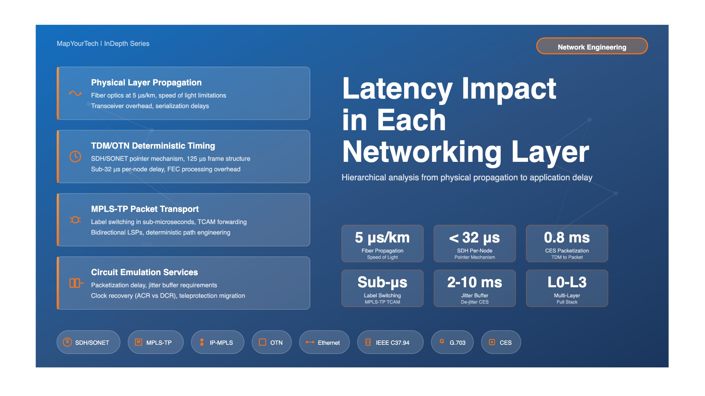
In optical fiber (single-mode fiber at 1550 nm wavelength), the refractive index is approximately 1.468, resulting in a propagation speed of approximately 204,217 km/s. This translates to approximately 4.9 microseconds of delay per kilometer of fiber. While copper cables have varying propagation speeds depending on insulation and construction, practical values fall in a similar range of 4.6 to 5.0 microseconds per kilometer.

1.2 Serialization Delay

Serialization delay (also called transmission delay) is the time required to place all bits of a data unit onto the physical transmission medium at a given link rate. Even with instantaneous propagation, a transmitter must serialize the packet bits sequentially onto the wire or fiber. This delay is directly proportional to the data unit size and inversely proportional to the link rate.

Serialization Delay = Packet Size (bits) / Link Rate (bits/second)

Example calculations:
• 1500-byte Ethernet frame at 100 Mbps: (1500 × 8) / 100,000,000 = 120 μs
• 1500-byte Ethernet frame at 1 Gbps: (1500 × 8) / 1,000,000,000 = 12 μs
• 1500-byte Ethernet frame at 10 Gbps: (1500 × 8) / 10,000,000,000 = 1.2 μs
    

Higher bandwidth links dramatically reduce serialization delay for a given packet size. Modern 100 Gbps interfaces achieve serialization delays below 200 nanoseconds for standard Ethernet frames. In TDM circuits, serialization is continuous and tied to the clock rate of the channel, making it a constant component of the circuit's fundamental latency characteristics.

1.3 Processing and Switching Delay

Processing delay encompasses the time networking equipment spends examining, classifying, and forwarding data. This includes hardware forwarding operations, protocol overhead processing, and any necessary transformations or encapsulations. The magnitude of processing delay varies significantly based on the network layer and equipment architecture.

In SDH/SONET multiplexers operating at Layer 1, data may be buffered until the next frame boundary (frame period of 125 microseconds) and then forwarded using the pointer mechanism, introducing a maximum delay of 32 microseconds per node. Modern packet routers using ASIC-based forwarding can process packets in microseconds, with label switching operations in MPLS networks often achieving sub-microsecond forwarding times.

Processing delay becomes highly variable in software-based forwarding, complex policy enforcement, or when packets require recirculation through processing pipelines. Network Address Translation, deep packet inspection, encryption/decryption, and traffic shaping all add processing overhead that can range from microseconds to milliseconds depending on implementation.

1.4 Queuing Delay

Queuing delay occurs when multiple data units arrive simultaneously for the same egress interface and must wait in buffers. This is the most variable component of network latency and depends heavily on network congestion, traffic patterns, and Quality of Service (QoS) configurations. Under low utilization, queuing delay may be negligible (microseconds). During congestion, queuing delay can dominate total latency, reaching hundreds of milliseconds.

The mathematical relationship between link utilization and queuing delay follows queuing theory. For an M/M/1 queue (Poisson arrivals, exponential service times, single server), average queuing delay equals 1/(μ-λ), where μ is the service rate and λ is the arrival rate. As utilization approaches 100 percent, queuing delay increases asymptotically toward infinity.

1.5 Jitter and Buffering

Jitter represents the variation in packet delay over time. In packet networks, if some packets experience longer delays (due to queuing or route changes), the inter-packet timing becomes irregular. Applications requiring steady data rates—such as emulated TDM circuits, voice calls, or real-time video—use jitter buffers to smooth this variability by holding incoming packets briefly to allow slower packets to catch up, ensuring continuous output.

However, jitter buffers directly increase end-to-end latency. A common sizing approach sets the buffer depth to twice the maximum expected packet delay variation (PDV). For networks with well-controlled PDV of 2-3 milliseconds, jitter buffers might add 4-6 milliseconds of latency. Networks with poor jitter performance may require 10-20 millisecond buffers, significantly impacting applications like teleprotection that require sub-10 millisecond total latency.

2. Physical Layer Latency: Copper versus Fiber

The physical transmission medium forms the foundation of network latency. Both copper and optical fiber propagate signals at speeds approaching but not reaching the speed of light in vacuum. Understanding the subtle differences and practical implications of each medium is essential for network design.

2.1 Copper Transmission Characteristics

In copper cables, electrical signals propagate through metallic conductors at speeds determined by the velocity factor of the cable, which depends on the dielectric material used for insulation. Typical velocity factors range from 0.60 to 0.90 times the speed of light in vacuum. For Category 6A twisted-pair cable commonly used in enterprise networks, the velocity factor is approximately 0.69, yielding a propagation speed of about 206,616 km/s or roughly 4.84 microseconds per kilometer.

However, copper transmission at high data rates introduces additional latency through the physical layer electronics. Modern 10GBASE-T Ethernet transceivers (10 Gbps over twisted-pair copper) employ complex Digital Signal Processing (DSP) and sophisticated line coding (128b/130b encoding) to overcome signal degradation and crosstalk at high frequencies. Research measurements indicate that 10GBASE-T Small Form-factor Pluggable (SFP+) transceivers can introduce as much as 2.6 microseconds of round-trip latency—300 times larger than the overhead of standard fiber optics at equivalent distances.

This electronic processing overhead effectively negates any theoretical propagation speed advantage copper might have over fiber at short distances. For latency-sensitive applications, fiber optics provides superior performance even in local-area network deployments.

2.2 Optical Fiber Transmission Characteristics

Optical fiber transmits data using light pulses guided through a glass or plastic core. In single-mode fiber operating at 1550 nm (the most common wavelength for long-distance telecommunications), the refractive index is approximately 1.468. This yields a propagation velocity of 204,217 km/s (68.2 percent of vacuum speed of light) or approximately 4.9 microseconds per kilometer.

Unlike copper, fiber-optic transceivers introduce minimal electronic delay. Standard SFP, SFP+, and QSFP optical transceivers typically add less than 100 nanoseconds of latency for optoelectronic conversion. Coherent optical transceivers used in high-capacity DWDM systems incorporate sophisticated DSP for chromatic dispersion compensation, polarization mode dispersion mitigation, and soft-decision Forward Error Correction (FEC), adding approximately 200-500 nanoseconds of processing delay.

2.3 Optical Network Components and Their Latency Contributions

For ultra-low-latency metro applications, some network operators disable FEC on short links where optical signal quality supports error-free transmission without coding gain. Transparent DWDM systems that avoid OTN digital wrapping provide the lowest latency path, limited only by fiber propagation and minimal amplifier delays.

3. Layer 1 Transport: SDH/SONET Deterministic Timing

Synchronous Digital Hierarchy (SDH) and its North American counterpart SONET represent the foundation of carrier-grade telecommunications networks. These Layer 1 transport technologies achieved their legendary reliability and determinism through rigid frame structures synchronized to an 8 kHz reference clock, producing frame periods of exactly 125 microseconds at all hierarchy levels.

3.1 The 125 Microsecond Framework

SDH/SONET systems achieve timing precision through synchronization to a Primary Reference Clock (PRC) with accuracy of ±1×10^-11. This creates networks where latency is not only low but perfectly predictable. Bandwidth in SDH is dedicated and fixed—an STM-1 circuit at 155.52 Mbps or an STM-16 circuit at 2.5 Gbps reserves its capacity regardless of whether data is being actively transmitted, ensuring constant and predictable latency characteristics.

The internal architecture of an SDH frame features byte-oriented multiplexing with overhead bytes (Section Overhead and Path Overhead) interleaved with payload in a complex structure. This interleaving is an intentional design that allows encapsulated data to "float" within the frame structure through the pointer mechanism, permitting very low transit delays.

3.2 Timing, Pointers, and Jitter Mechanisms

SDH handles small frequency and phase differences between network nodes through Administrative Unit (AU) and Tributary Unit (TU) pointers (bytes H1, H2, and H3). These pointers identify where the payload begins within the frame. If an incoming signal's clock is slightly faster or slower than the local node's clock, the pointer value adjusts, effectively shifting the payload by one byte to maintain synchronization without data loss.

Sanjay Yadav

Optical Communications & Network Automation Expert | Author of 3 Books for Optical Engineers | Founder, MapYourTech

Optical networking engineer with nearly two decades of experience across DWDM, OTN, coherent optics, submarine systems, and cloud infrastructure. Founder of MapYourTech. Read full bio →

Follow on LinkedIn

Related Articles on MapYourTech

Coherent Optics · Jul 10, 2026

The Submarine Cable Stack: Open Cables, Generalized OSNR, SDM and Power-Constrained Transmission

Coherent Optics · Jul 10, 2026

Coherent DSP Architecture: From ADC Samples to Client Bits

Automation · Jul 10, 2026

Building an Optical NOC Dashboard with OpenConfig Telemetry

Coherent Optics · Jul 10, 2026

Spectral Efficiency in Practice: The Four Levers